A Primer On Evaluation Techniques In Data Science Classification Methods

With the growth of data, tools and techniques to do predictive modelling as well as the evaluation methods used to assess the performance of a model have evolved. Model development is an iterative process and evaluation methods play an important role in it.

Machine learning has two key parts — supervised and unsupervised. This article will focus on evaluation methods used for supervised machine learning wherein we predict the target using labelled data. We will focus on classification and regression models in supervised machine learning category.

A Typical Machine Learning Process

The evaluation stage is the most critical one. It’s a good practice to decide in advance which evaluation matrix will be used to evaluate the performance of a model because this is the stage which will help decide if the model is acceptable.

So how do we decide which evaluation matrix to use for a model? Does it depend on the technique or business problem? Let’s explore.

Evaluation Methods for Classification

For classification problems, we will look at the 2×2 confusion matrix.

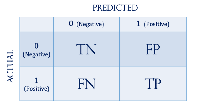
TP: Actual true and predicted true

TN: Actual false and predicted false

FP: Actual false and predicted true

FN: Actual true and predicted false

A few matrices can be calculated using the confusion matrix

• Accuracy: (TP+TN)/Total
• Misclassification: (FP+FN)/total or (1-Accuracy)
• Precision: TP/(TP+FP). Out of total predicted true, what is the % of actual true as in how often model predicts accurately
• Recall/ Sensitivity/TPR: TP/(TP+FN). How sensitive the model is to predict an actual value of a true.
• False Positive Rate (FPR)/Specificity: FP/(FP+TN)
• F1: (2*Recall*Precision)/(Recall+Precision)

Let’s look at an example:

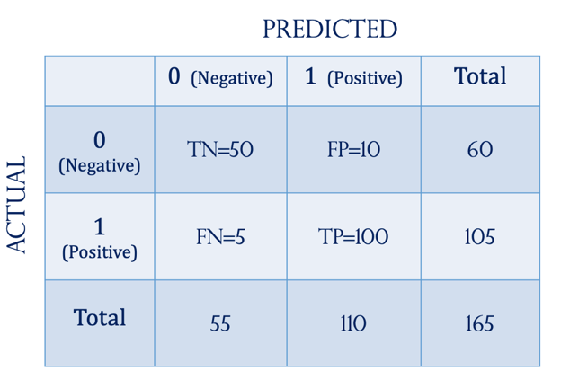
1. Accuracy=91%

Accuracy is not always the right method to measure performance. Example, in credit card transactions vast majority of transactions (e.g.99 out of 100) will be non-fraudulent. If we used accuracy to predict a non-fraudulent transaction, it’s going to be close to 99% and this is not correct. Imbalance classes are very common in machine learning scenarios and hence accuracy might not always be the right evaluation method.

2. Recall/Sensitivity/TPR=95%

High recall means not only accurately predicted TP but also avoided false negatives. In cancer detection example, it would mean it not only detected a high number for TP as in identifying people who have cancer correctly but also it rarely failed to detect a true cancer. If the objective is to increase Recall then either increase TP or reduce FN.

3. Precision=91%

It’s acceptable that all not all true positives are correct but when detected it must be correct. For example, we want to send a customer a recommendation to buy a savings product through an email and we need to make that it is relevant for the customer — a customer remembers incorrect marketing and will not be a good experience. If we want to increase precision, we either increase TP or reduce FP.

4. Specificity/FPR=17%

A fraction of all negative instances that the classifier incorrectly identifies as positive. In other words, out of a total number of actual negatives, how many instances the model falsely classifies as non-negative.

Graphical Evaluation Methods

Precision-Recall curve

Precision-Recall curve provides visualised information at various threshold levels. 

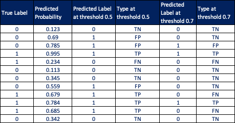
Below, we have 12 records for actual/true labels, probability, predicted label at threshold 0.5 and 0.7.

As threshold changes, predicted label changes which effects Recall and Precision.

We use different cutoffs or thresholds to derive values for precision and recall which are plotted on a graph which is called Precision-Recall curve. 

An ideal point for a precision-recall curve is the top right corner where both Precision and Recall are equal to 1, meaning there are no FP and no FN. However, in the real world this is highly unlikely, so any point closer to the top right corner will be an ideal point. 

ROC and AUC (Area Under the Curve)

ROC curve uses a False Positive rate (FPR) and True Positive Rate (TPR). An ideal point is a top left corner where TPR is 1 and FPR is 0, meaning there are no FN and no FP. For ROC, we should look to maximise TPR while minimising FPR.

AUC can be derived from ROC curve which measures the area underneath the ROC curve to summarise a classifier’s performance. The area under the dotted straight line is 0.5 which represents random guess — just like flipping coin results in 2 outcomes. An AUC of zero represents a very bad classifier, and an AUC of 1 will represent an optimal classifier.

Conclusion

One model does not fit all types of data, hence it’s important that we set a single number evaluation method at the start, so that we can quickly evaluate the performance and move to the option which is working the best.