


Visual exploration can be said as one of the crucial components of data analysis. Visualisation of high-dimensional datasets can be said as one of the major tasks in several domains. In this article, we will help you understand the basic of t-SNE and it’s weaknesses.
Stochastic Neighbour Embedding (SNE) locates the objects in a low-dimensional space to optimally preserve neighbourhood identity and starts by converting the high-dimensional Euclidean distances between data-points into conditional probabilities which represent similarities. It can also be applied to datasets which consist of pairwise similarities between objects rather than high-dimensional vector representation of each object, provided these similarities can be interpreted as conditional probabilities.
The drawbacks of SNE are that it is hampered by a cost function which is difficult to optimise along with the “crowding problem”. These shortcomings can be overcome by t-SNE as t-SNE employs a heavy-tailed distribution in the low-dimensional space to alleviate both the crowding problem and the optimization problems of SNE. The cost function used by t-SNE is different from the one used by SNE. The difference is basically by two ways as mentioned below
- It uses a symmetrised version of the SNE cost function with simpler gradients
- It uses a Student-t distribution rather than a Gaussian to compute the similarity between two points in the low-dimensional space
t-Distributed Stochastic Neighbour Embedding (t-SNE) is a machine learning technique for dimensionality reduction which is well-suited for visualisation of high-dimensional datasets. It visualises high-dimensional data by giving each data-point a location in a two or three-dimensional map. It is a valuable tool in generating hypothesis and understanding.
t-SNE generally produces maps which provide a clearer insight into the underlying structure of the data with the help of the two mentioned characteristics
- t-SNE mainly focuses on appropriately modeling small pairwise distances, i.e. local structure, in the map
- t-SNE has a way to correct for the enormous difference in the volume of high-dimensional feature space and a two-dimensional map
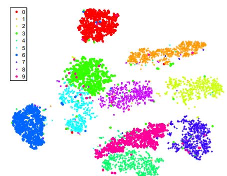
Fig: Visualisation by t-SNE on MNIST dataset
Do’s And Don’ts
There are several dos and don’ts one must follow while using the t-SNE technique. Some of them are mentioned below
- t-SNE can be used to get qualitative hypothesis on what the features captured.
- Scale (perplexity) matters as it can be considered as the effective number of nearest neighbours.
- It is ok to run t-SNE multiple times in order to pick the best solution.
- Do not present proof by t-SNE since the visualised map is not data.
- Do not forget to consider an alternative hypothesis
- Do not assign meaning to the distances across empty space
- Do not think that t-SNE will help to find an outlier, or assign meaning or point densities in clusters
- Do not forget that t-SNE minimises a non-convex objective as there are local minima which generally split a natural cluster into multiple parts
Vulnerabilities
t-SNE can be compared fairly to other techniques for data visualisation. But this tool has three potential vulnerabilities as mentioned below
- Dimensionality Reduction for other purposes: It is uncertain on how t-SNE performs on general dimensionality reduction tasks i.e. when the dimensionality of the data is not reduced to two or three, but to d > 3 dimensions.
- Curse of intrinsic dimensionality: In data sets with high intrinsic dimensionality and an underlying manifold which is highly varying, the local linearity assumption on the manifold which t-SNE implicitly makes may be violated. t-SNE reduces the dimensionality of data mainly based on local properties of the data, which makes t-SNE sensitive to the curse of the intrinsic dimensionality of the data.
- Non-convexity of the t-SNE cost function: A major weakness of t-SNE is that the cost function is not convex, as a result of which several optimization parameters need to be chosen.