ODE2VAE, a representation learning model, achieves state-of-the-art performance in long-term motion prediction and imputation tasks. It is introduced as a generative latent second-order Ordinary Differential Equation model for high dimensional sequential data such as motion capture. Variational autoencoders (VAE) are well known for their ability to extract hidden patterns from image data. VAE based models or their extensions usually assume static data. Hence VAE is not suitably applicable to sequential data, which are dynamic. ODE2VAE is a breakthrough in applying VAE to sequential data with latent space controlled by a continuous-time probabilistic second order ODE.
The model proposes a second-order ODE that permits modelling the latent dynamic ODE state, which decomposes high dimensional space into positions and momentum. To handle the uncertainty in the dynamics, the Bayesian neural network is introduced to the dynamics model. ODE2VAE performs state-of-the-art performance in all levels of learning with the variational inference approach, reproducing and forecasting high dimensional image sequential systems. Recurrent neural networks based VAE models can forecast a single step future image, but not a sequence of future images, whereas ODE2VAE predicts long-term future sequences with better accuracy than any of the well-known models.
First-order ODEs are incapable of modelling high-order dynamics such as acceleration or the motion of a pendulum. On the other hand, ODEs are deterministic systems unable to account for uncertainties in the dynamics. But ODE2VAE tackles both issues by introducing Bayesian neural second-order ODEs.
Illustration of dynamical systems. (a) A continuous-time system underlying a discrete-time model, (b) Extended to a 2nd-order ODE with velocity component, (c) A Bayesian ODE characterizes uncertain differential dynamics, and (d) The corresponding position-velocity phase-diagram with arrows in indicating the Bayesian Neural Network field.
As a generative model, ODE2VAE consists of three components: first, the distribution of initial position and velocity; second, true dynamics defined by the acceleration field; third, a decoding likelihood.
Positional encoder maps the first example of high dimensional input sequence into a distribution of initial position in latent space. Velocity encoder maps a set of input sequence examples into a distribution of initial velocity in a latent space. Probabilistic latent dynamics are implemented by a second order ODE model parameterized by a Bayesian deep neural network. Data points in the original data domain are reconstructed by a decoder based on the parameters of time, position and velocity.
TensorFlow implementation of ODE2VAE
ODE2VAE is presently released as both TensorFlow implementation and PyTorch implementation. To obtain the package, we need to install the necessary libraries and dependencies with versions specified below.
 %%bash
 cd ODE2VAE
 ./scripts/train_mnist.sh
 ./scripts/test_mnist.sh
To run the pre-trained walking sequences script and its test script,
 %%bash
 cd ODE2VAE
 ./scripts/train_mocap_single.sh
 ./scripts/test_mocap_single.sh
To run the pre-trained multiple-walking sequences script and its test script,
 %%bash
 cd ODE2VAE
 ./scripts/train_mocap_many.sh
 ./scripts/test_mocap_many.sh
PyTorch Implementation of ODE2VAE
For PyTorch implementation, we need to install the following packages additionally,
 %%bash
 pip install torch
 pip install torchdiffeq
Simple and complete python code implementation can be realized by importing the following libraries and modules.
 import torch
 import torch.nn as nn
 import torch.nn.functional as F
 from torch.nn.parameter import Parameter
 from torch.utils import data
 from torch.distributions import MultivariateNormal, Normal, kl_divergence as kl
 from torch_bnn import BNN
 device = torch.device('cuda' if torch.cuda.is_available() else 'cpu')
 from torchdiffeq import odeint
 import numpy as np
 from scipy.io import loadmat
 import matplotlib.pyplot as plt
 plt.switch_backend('agg')
 import os
 os.environ['KMP_DUPLICATE_LIB_OK']='True'
 from multiprocessing import Process, freeze_support
 torch.multiprocessing.set_start_method('spawn', force="True")
Loading and Preprocessing of data can be done with
Define some useful classes to flatten and unflatten the views
 class Flatten(nn.Module):
     def forward(self, input):
         return input.view(input.size(0), -1)
 class UnFlatten(nn.Module):
     def __init__(self,w):
         super().__init__()
         self.w = w
     def forward(self, input):
         nc = input[0].numel()//(self.w**2)
         return input.view(input.size(0), nc, self.w, self.w)
Finally, the VAE modelling class is developed with the code.
 class ODE2VAE(nn.Module):
     def __init__(self, n_filt=8, q=8):
         super(ODE2VAE, self).__init__()
         h_dim = n_filt*4**3 # encoder output is [4*n_filt,4,4]
         # encoder
         self.encoder = nn.Sequential(
             nn.Conv2d(1, n_filt, kernel_size=5, stride=2, padding=(2,2)), # 14,14
             nn.BatchNorm2d(n_filt),
             nn.ReLU(),
             nn.Conv2d(n_filt, n_filt*2, kernel_size=5, stride=2, padding=(2,2)), # 7,7
             nn.BatchNorm2d(n_filt*2),
             nn.ReLU(),
             nn.Conv2d(n_filt*2, n_filt*4, kernel_size=5, stride=2, padding=(2,2)),
             nn.ReLU(),
             Flatten()
         )
         self.fc1 = nn.Linear(h_dim, 2*q)
         self.fc2 = nn.Linear(h_dim, 2*q)
         self.fc3 = nn.Linear(q, h_dim)
         # differential function
         # to use a deterministic differential function, set bnn=False and self.beta=0.0
         self.bnn = BNN(2*q, q, n_hid_layers=2, n_hidden=50, act='celu', layer_norm=True, bnn=True)
         # downweighting the BNN KL term is helpful if self.bnn is heavily overparameterized
         self.beta = 1.0 # 2*q/self.bnn.kl().numel()
         # decoder
         self.decoder = nn.Sequential(
             UnFlatten(4),
             nn.ConvTranspose2d(h_dim//16, n_filt*8, kernel_size=3, stride=1, padding=(0,0)),
             nn.BatchNorm2d(n_filt*8),
             nn.ReLU(),
             nn.ConvTranspose2d(n_filt*8, n_filt*4, kernel_size=5, stride=2, padding=(1,1)),
             nn.BatchNorm2d(n_filt*4),
             nn.ReLU(),
             nn.ConvTranspose2d(n_filt*4, n_filt*2, kernel_size=5, stride=2, padding=(1,1), output_padding=(1,1)),
             nn.BatchNorm2d(n_filt*2),
             nn.ReLU(),
             nn.ConvTranspose2d(n_filt*2, 1, kernel_size=5, stride=1, padding=(2,2)),
             nn.Sigmoid(),
         )
         self._zero_mean = torch.zeros(2*q).to(device)
         self._eye_covar = torch.eye(2*q).to(device)
         self.mvn = MultivariateNormal(self._zero_mean, self._eye_covar)
     def ODE2VAE_rhs(self,t,vs_logp,f):
         vs, logp = vs_logp # N,2q & N
         q = vs.shape[1]//2
         dv = f(vs) # N,q
         ds = vs[:,:q]  # N,q
         dvs = torch.cat([dv,ds],1) # N,2q
         ddvi_dvi = torch.stack(
                     [torch.autograd.grad(dv[:,i],vs,torch.ones_like(dv[:,i]),
                     retain_graph=True,create_graph=True)[0].contiguous()[:,i]
                     for i in range(q)],1) # N,q --> df(x)_i/dx_i, i=1..q
         tr_ddvi_dvi = torch.sum(ddvi_dvi,1) # N
         return (dvs,-tr_ddvi_dvi)
     def elbo(self, qz_m, qz_logv, zode_L, logpL, X, XrecL, Ndata, qz_enc_m=None, qz_enc_logv=None):
         [N,T,nc,d,d] = X.shape
         L = zode_L.shape[0]
         q = qz_m.shape[1]//2
         # prior
         log_pzt = self.mvn.log_prob(zode_L.contiguous().view([L*N*T,2*q])) # L*N*T
         log_pzt = log_pzt.view([L,N,T]) # L,N,T
         kl_zt   = logpL - log_pzt  # L,N,T
         kl_z    = kl_zt.sum(2).mean(0) # N
         kl_w    = self.bnn.kl().sum()
         # likelihood
         XL = X.repeat([L,1,1,1,1,1]) # L,N,T,nc,d,d
         lhood_L = torch.log(1e-3+XrecL)*XL + torch.log(1e-3+1-XrecL)*(1-XL) # L,N,T,nc,d,d
         lhood = lhood_L.sum([2,3,4,5]).mean(0) # N
         if qz_enc_m is not None: # instant encoding
             qz_enc_mL    = qz_enc_m.repeat([L,1])  # L*N*T,2*q
             qz_enc_logvL = qz_enc_logv.repeat([L,1])  # L*N*T,2*q
             mean_ = qz_enc_mL.contiguous().view(-1) # L*N*T*2*q
             std_  = 1e-3+qz_enc_logvL.exp().contiguous().view(-1) # L*N*T*2*q
             qenc_zt_ode = Normal(mean_,std_).log_prob(zode_L.contiguous().view(-1)).view([L,N,T,2*q])
             qenc_zt_ode = qenc_zt_ode.sum([3]) # L,N,T
             inst_enc_KL = logpL - qenc_zt_ode
             inst_enc_KL = inst_enc_KL.sum(2).mean(0) # N
             return Ndata*lhood.mean(), Ndata*kl_z.mean(), kl_w, Ndata*inst_enc_KL.mean()
         else:
             return Ndata*lhood.mean(), Ndata*kl_z.mean(), kl_w
     def forward(self, X, Ndata, L=1, inst_enc=False, method='dopri5', dt=0.1):
         # encode
         [N,T,nc,d,d] = X.shape
         h = self.encoder(X[:,0])
         qz0_m, qz0_logv = self.fc1(h), self.fc2(h) # N,2q & N,2q
         q = qz0_m.shape[1]//2
         # latent samples
         eps   = torch.randn_like(qz0_m)  # N,2q
         z0    = qz0_m + eps*torch.exp(qz0_logv) # N,2q
         logp0 = self.mvn.log_prob(eps) # N
         # ODE
         t  = dt * torch.arange(T,dtype=torch.float).to(z0.device)
         ztL   = []
         logpL = []
         # sample L trajectories
         for l in range(L):
             f       = self.bnn.draw_f() # draw a differential function
             oderhs  = lambda t,vs: self.ODE2VAE_rhs(t,vs,f) # make the ODE forward function
             zt,logp = odeint(oderhs,(z0,logp0),t,method=method) # T,N,2q & T,N
             ztL.append(zt.permute([1,0,2]).unsqueeze(0)) # 1,N,T,2q
             logpL.append(logp.permute([1,0]).unsqueeze(0)) # 1,N,T
         ztL   = torch.cat(ztL,0) # L,N,T,2q
         logpL = torch.cat(logpL) # L,N,T
         # decode
         st_muL = ztL[:,:,:,q:] # L,N,T,q
         s = self.fc3(st_muL.contiguous().view([L*N*T,q]) ) # L*N*T,h_dim
         Xrec = self.decoder(s) # L*N*T,nc,d,d
         Xrec = Xrec.view([L,N,T,nc,d,d]) # L,N,T,nc,d,d
         # likelihood and elbo
         if inst_enc:
             h = self.encoder(X.contiguous().view([N*T,nc,d,d]))
             qz_enc_m, qz_enc_logv = self.fc1(h), self.fc2(h) # N*T,2q & N*T,2q
             lhood, kl_z, kl_w, inst_KL = \
                 self.elbo(qz0_m, qz0_logv, ztL, logpL, X, Xrec, Ndata, qz_enc_m, qz_enc_logv)
             elbo = lhood - kl_z - inst_KL - self.beta*kl_w
         else:
             lhood, kl_z, kl_w = self.elbo(qz0_m, qz0_logv, ztL, logpL, X, Xrec, Ndata)
             elbo = lhood - kl_z - self.beta*kl_w
         return Xrec, qz0_m, qz0_logv, ztL, elbo, lhood, kl_z, self.beta*kl_w
     def mean_rec(self, X, method='dopri5', dt=0.1):
         [N,T,nc,d,d] = X.shape
         # encode
         h = self.encoder(X[:,0])
         qz0_m = self.fc1(h) # N,2q
         q = qz0_m.shape[1]//2
         # ode
         def ODE2VAE_mean_rhs(t,vs,f):
             q = vs.shape[1]//2
             dv = f(vs) # N,q
             ds = vs[:,:q]  # N,q
             return torch.cat([dv,ds],1) # N,2q
         f     = self.bnn.draw_f(mean=True) # use the mean differential function
         odef  = lambda t,vs: ODE2VAE_mean_rhs(t,vs,f) # make the ODE forward function
         t     = dt * torch.arange(T,dtype=torch.float).to(qz0_m.device)
         zt_mu = odeint(odef,qz0_m,t,method=method).permute([1,0,2]) # N,T,2q
         # decode
         st_mu = zt_mu[:,:,q:] # N,T,q
         s = self.fc3(st_mu.contiguous().view([N*T,q]) ) # N*T,q
         Xrec_mu = self.decoder(s) # N*T,nc,d,d
         Xrec_mu = Xrec_mu.view([N,T,nc,d,d]) # N,T,nc,d,d
         # error
         mse = torch.mean((Xrec_mu-X)**2)
         return Xrec_mu,mse
 # plotting
 def plot_rot_mnist(X, Xrec, show=False, fname='rot_mnist.png'):
     N = min(X.shape[0],10)
     Xnp = X.detach().cpu().numpy()
     Xrecnp = Xrec.detach().cpu().numpy()
     T = X.shape[1]
     plt.figure(2,(T,3*N))
     for i in range(N):
         for t in range(T):
             plt.subplot(2*N,T,i*T*2+t+1)
             plt.imshow(np.reshape(Xnp[i,t],[28,28]), cmap='gray')
             plt.xticks([]); plt.yticks([])
         for t in range(T):
             plt.subplot(2*N,T,i*T*2+t+T+1)
             plt.imshow(np.reshape(Xrecnp[i,t],[28,28]), cmap='gray')
             plt.xticks([]); plt.yticks([])
     plt.savefig(fname)
     if show is False:
         plt.close()
# calling the program to run
if __name__ == '__main__':
freeze_support()
ODE2VAE = ODE2VAE(q=8,n_filt=16).to(device)
Nepoch = 500
optimizer = torch.optim.Adam(ODE2VAE.parameters(),lr=1e-3)
for ep in range(Nepoch):
L = 1 if ep
It is advisable to train or evaluate the CUDA GPU runtime implementations, though the code can be run in CPU runtime.
Performance evaluation
With the rotating mnist digits dataset, ODE2VAE can reconstruct the sequence of rotating images of digits with great performance.
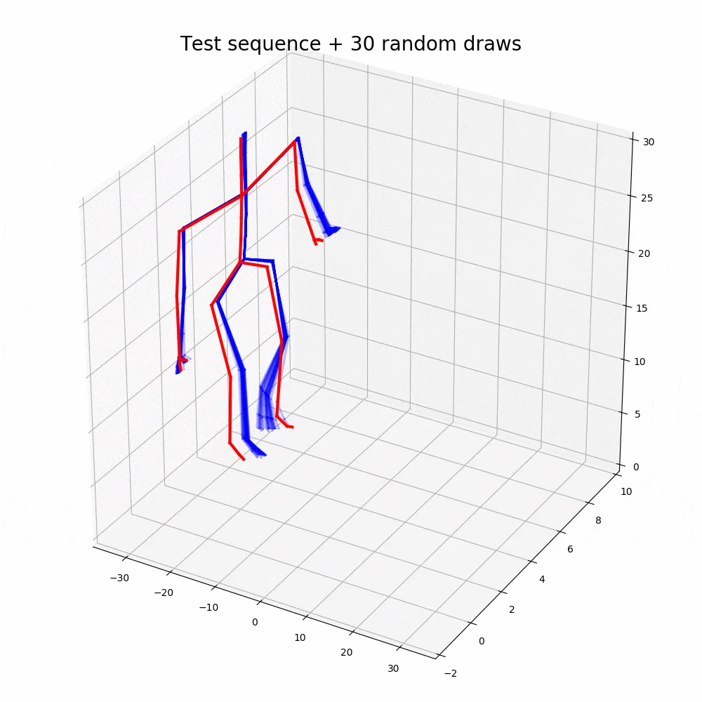
With the walking sequences dataset, the model can reconstruct the sequence with greater performance than any other representation learning algorithm.
Comparison of predictive mean square errors caused by the ODE2VAE with that of DDPAE and DTSBN-S models with bouncing balls datasetThe reconstruction of bouncing balls image sequences - comparison among the various models
Based on the performance, it is clear that the ODE2VAE outperforms any of the models in sequence reconstruction such as Gaussian Process Dynamic Models (GPDM), Variational Gaussian Process Dynamical Systems (VGPLVM), Deep Temporal Sigmoidal Belief Networks for Sequence Modeling (DTSBN-S), Gaussian Process Ordinary Differential Equation (npODE), Neural Ordinary Differential Equations (NeuralODE).



Your reaction
Discussion
What's your take on this story?
No comments yet — be the first to share your view.