‘Expectation Maximisation’ Explained With A Coin Toss

Parameter estimation is the process of using training data to estimate or calculate parameters of selected distributions. Many techniques like least square methods, probability plotting and other advanced methods like maximum likelihood estimation and expectation maximisation are encompassed in this general definition. There are many techniques that can estimate model parameters from latent unobserved variables. But the expectation maximisation (EM) algorithm is one of the most popular and useful parameter estimation technique.

Setting Up The Problem

When working on a very new problem you come across some data that does not have any labels. Here, one has to guess (assume) the distribution and then come up with a hypothesis to find the parameters of that distribution. Let us consider this example:

There are two coins that need to be flipped and the sequence of flipping results need to be captured. It looks something like this:

If it is a fair coin, then the probability of heads coming up as a parameter θ is 0.5. If the probability of heads is higher than the value of θ, it will be over this number. And it will be lower if the probability of heads is very low. A simple way to understand this is:

Number of Heads / Number of Heads + Number of Tails

Doing Better A Job At Estimation

Imagine that the above simple calculation is done for two coins A and B. Let us call the parameter estimates to be θA and θB. We call these the maximum likelihood values and they are responsible for the distribution that came up during the experimentation. In a way, you can imagine these parameters to be the values that maximise the likelihood of getting a particular distribution for A and B. This is the idea behind the likelihood function which serves the purpose of telling us that given some data and parameters (and a distribution) how well the parameters explain the data. It is the ultimate test to know if we reached a correct set of parameters. In the case of the coin flip, we take the binomial formula as the likelihood function. It can be represented as:

Since all we care about is the maximisation of θ, we can ignore other constants in that process. Hence we aim to maximise the expression θH(1−θ)T . We assume that k is constant because the prior as constant. There is no limitation on a likelihood function like a probability function where the values have to lie between 0 and 1.

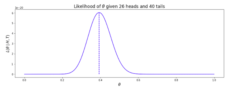
Now the likelihood can be given as: L(θ / H,T) = θH(1−θ)T

If we plot the θ for values between 0 and 1 we get a similar maximum likelihood value similar to what we get programmatically.

Expectation Maximisation

Imagine now that the labels for the data are gone. It means that the data is all mixed. The data is now mixed and now we can’t separate the data from the two. Here is where Expectation Maximisation comes into play. The steps involved in EM algorithms are:

1. Guess the random initial estimates of θA and θB between 0 and 1.
2. Use the likelihood function use the parameter values to see how probable the data is.
3. Use this likelihood to generate a weighting for indicating the probability of each sequence produced using θA and θB. This is called the Expectation Step.
4. Add up the total number of weighted counts for heads and tails across all sequences (call these counts H′ and T′) for both parameter estimates. Produce new estimates for θA and θB using the maximum likelihood formula H′ / H′+T′ (the Maximisation step).
5. Repeat steps 2-4 until each parameter estimate has converged, or a set number of iterations has been reached. The total weight for each sequence should be normalised to 1.

EM may also tend to switch the parameter values between two coins.

Why EM works

With EM the parameters magically improve with each iteration and eventually converge. It is so because each data point is associated with a weight during each iteration of the EM algorithm. It shows us the how the parameters explain the data and if the newest parameters fit the data well. Sum of weights is always maintained to 1. Expectation set tells us how different data points contribute to the newly calculated maximum likelihood estimate which was calculated during the last maximisation step.

In the subsequent iterations, we need to find the likelihood that the data was generated by θA. If it greater than before, even greater weight is given for the particular data sequence. Since the sum of the weights can’t be more than 1 the weights converge towards 1 eventually.