


In Recent times, Deep learning has seen increased demand by the tech communities in the field of computer vision. In our day to day life, we are always surrounded by the applications of Deep learning, from high-tech mobile phones to driverless cars, there are a lot of applications which help us in everyday life.
Through this article, we will demonstrate the implementation of HarDNet – a deep learning framework – using pre-trained weights which are already trained on ImageNet dataset. The ImageNet dataset is a popular benchmark dataset in computer vision with 1000 class labels. We will use the PyTorch framework for the implementation of our model. In our implementation, we will take a random image of a dog, and the HarDNet model will recognize it with its breed.
Topics We Cover
- Introduction to HarDNet
- Architecture of HarDNet Model
- Why do we need HarDNet?
- Implementation of Hardnet using Pytorch
- Object Recognition using HarDNet
Introduction to HarDNet
HarDNet is referred to as A LOW MEMORY TRAFFIC NETWORK. In the past few years, computer vision has seen a huge improvement in terms of computational efficiency and huge datasets that made possible training complex networks. But to work on real-time applications, the main issue was we need to increase computational efficiency and reduce the power consumption. So to solve this problem researchers had their first step to maintaining the balance between increasing computational efficiency & to reduce the power consumption.
Architecture of HarDNet
HarDNet is an image classification network belonging to the category of deep learning models. We can use HarDNet for the task of image segmentation and object detection. The architecture was based on Densely Connected Network. In HarDNet, we have multiple Harmonic Dense Blocks, so what are Harmonic Dense blocks ………….???? In Harmonic Blocks we have n layers and each block is connected to its preceding blocks, hence the last layer has the largest number of channels because all previous layers outputs are forwarded to preceding layers. Not only the forward connection we also move backwards, let layer k connect to layer k-(2)n, once layer (2)n is processed then flushes out the memory.
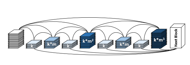
By referring to the figure given above, we can see that the network appears as an overlapping of harmonic waves. The other name of HarDNet was Harmonic Densely Connected Network, in short, we call it as HarDNET.
Here we have the 4 versions of HarDNet models, which contains 39, 68, 85 layers with and without Depthwise Separable Conv respectively. Their 1-crop error rates on ImageNet dataset with pre-trained models are listed below.
| Model structure | Top-1 error | Top-5 error |
| HarDNet39ds | 27.92 | 9.57 |
| HarDNet68ds | 25.71 | 8.13 |
| HarDNet68 | 23.52 | 6.99 |
| HarDNet85 | 21.96 | 6.11 |
Why We Need HarDNet Over Other Networks
We have many image classification algorithms but compared to other classification algorithms, HarDNet reduces the power and achieves similar accuracy. Popular object detection SSD uses HarDNet-68 as the backbone which is a state of art and we can use HarDNet for Segmentation tasks for downsampling the image.
Implementation of HarDNet In PyTorch
Here we are going to use PyTorch, so let’s have a brief introduction about PyTorch. It was developed by Facebook AI team and it provides a good interface for researchers, for more details, please visit this link.
Here, we are using Google Colab for implementing our code. The Google Colab provides free GPU and TPU hardware support that’s the reason why most of the researchers prefer to use Colab. By opening Google Colab and visiting the Notebook Settings in Edit Menu, we can change the hardware accelerator set to GPU. You can refer to the below image.

In the below block of code, we will load pre-trained weights for HarDNet with the different number of layers and for Depth wise separable convolutions.
import torch
model = torch.hub.load('PingoLH/Pytorch-HarDNet', 'hardnet68', pretrained=True)
model.eval()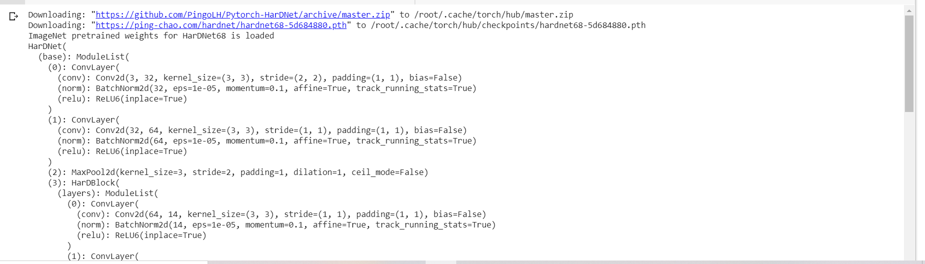
Here in the output above, you can see the pre-trained weights gets loaded.
In the next step, we will load an image for the task of object detection.
import urllib
url, filename = ("the url which we have image")
try: urllib.URLopener().retrieve(url, filename)
except: urllib.request.urlretrieve(url, filename)
Using below code snippet will read the URL from the image.
import urllib
url, filename = ("https://github.com/pytorch/hub/raw/master/dog.jpg", "dog.jpg")
try: urllib.URLopener().retrieve(url, filename)
except: urllib.request.urlretrieve(url, filename)
By using below code snippet we can visualize the image.
from PIL import Image
img = Image.open("dog.jpg")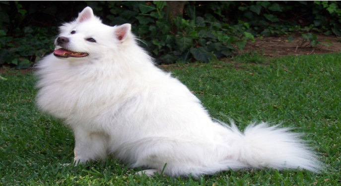
By using the below code snippet, we will perform the transformations of the image. As we are going to implement this task in PyTorch, and the basic unit PyTorch is a tensor, so we will transform the input data into the tensor.
from PIL import Image
from torchvision import transforms
input_image = Image.open(filename)
preprocess = transforms.Compose([
    transforms.Resize(256),
    transforms.CenterCrop(224),
    transforms.ToTensor(),
    transforms.Normalize(mean=[0.485, 0.456, 0.406], std=[0.229, 0.224, 0.225]),
])
input_tensor = preprocess(input_image)
input_batch = input_tensor.unsqueeze(0) # create a mini-batch as expected by the model
Object Recognition using HarDNet in PyTorch
Using the below code snippet we will download the labels of the ImageNet dataset and store it in classes.
with open('/content/imagenet1000_clsidx_to_labels.txt') as f:
  classes = [line.strip() for line in f.readlines()]
print(classes)
Using the below code snippet we will obtain the top 5 confidence classes to which the detected object may belong to.
#Moving the model to CUDA
if torch.cuda.is_available():
    input_batch = input_batch.to('cuda')
    model.to('cuda')

with torch.no_grad():
    output = model(input_batch)
_, indices = torch.sort(output, descending=True)
percentage = torch.nn.functional.softmax(output, dim=1)[0] * 100
[(classes[idx], percentage[idx].item()) for idx in indices[0][:5]]
We can see in the output obtained above that we have got 97.7 confidence score for Samoyed breed and for the white wolf, Arctic wolf, we have got 0.88 confidence score. So, we have achieved good confidence score for Samoyed breed.
Conclusion
So we conclude the HarDNet model has applied in the task of object recognition and it recognized the object with 97.7 confidence score. HarDNet is used to minimize both computational cost and memory access cost without compromising the accuracy. Through this article, we have learnt about HarDNet in PyTorch, it’s architecture, its importance and its application in object recognition.