


In this article, we will see how the Taylor series can help us simplify functions like cos(θ) into polynomials for ease of computation.
Taylor series is a modified version of the Maclaurin series introduced by Brook Taylor in the 18th century. Taylor series of a function is an infinite sum of terms that are expressed in terms of the function’s derivatives at a single point. Converting a function to a Taylor Polynomial makes it easier to deal with. Firstly, let’s look at an example to derive a Maclaurin series for cos(θ).
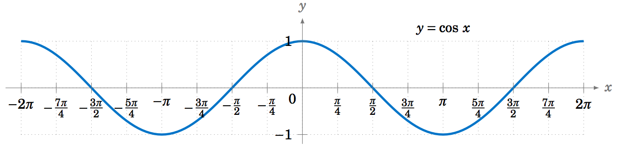
The above-given graph is for y = cos(θ). This function can be converted to a Maclaurin Series by following certain rules.
To resemble the same graph for a series, we must make sure that the Maclaurin series should inherit some characteristics from the function, cos(θ). Firstly, let’s check for the value of cos(x) at x=0.
Cos(0) = 1. Now that we have the value of cos(x) at 0, we must try and get the same property for our new Maclaurin series. Let’s work out the example by hand.

To resemble the behaviour of cos(x) in the Maclaurin series, C0 will be 1. This was the very first check to make sure that the value of the series and cos(x) is equal at x=0. Getting the same value for the Maclaurin series at x=0 does not mean our job is done. Let’s look at a visualization to understand what we have achieved till now.

All the dotted lines could be potential graphs of our Maclaurin series after setting the value of x=0. Essentially, we have managed to lock the series in a particular position. For better approximation, the next step will be replicating the slope of cos(x) at x=0 for the Maclaurin Series.

C1 should be equal to 0 to match the slope at cos(0). Therefore C1 = 0 and the series looks like this,

Furthermore, we need to try and fit the series equation to cos(x) to replicate the function. To do this we will take the help of higher-order derivatives. Let’s start by taking a second-order derivative of cos(x) and look at the value. The second-order derivative will give us the direction of the decreasing slope and will help the series curve in the correct direction.

This tells us that in order to follow the trajectory of cos(x) beyond x=0, the second order derivative of our series should be equal to -1.

If C2 = -1/2, then the equation will look like px=1-12 x2
Let’s try by comparing the value of cos(0.1) which is approximately equal to 0.995 and if we try p(0.1) we will get 0.995. This gives us a very good approximation. You could keep on adding terms to the series and try to get the best fit for the function but after a point the graph might start deviating from the original function. It is not necessary the series will converge entirely. The graph of the Maclaurin series could converge only in a certain region. What if we had more than three terms in our series? Something like,

So now even after adding a cubic term we are left with the same equation, which is
px=1-12 x2
Similarly let’s add a biquadratic term (degree 4). Therefore, our computations will look like,

If you look closely, the series follows a pattern, and it can be written as


So, the general form for the Maclaurin series is,

General form for Taylor series can be derived from the above formula. Taylor series is a modification of the Maclaurin series giving you the ability to select any arbitrary point besides 0.


Figure 3 General form for Taylor Series
Here “a” is the arbitrary point that you select. Having defined what a Taylor series is, we also need to think about the convergence of the series. The generated series might be convergent in an interval and divergent in the other. The distance from the selected arbitrary point “a” and the point where the series violates convergence is known as the radius of convergence.
Here are some most derived Taylor series.

Applications of Taylor Series:
- Physicists use Taylor series to test the approximation of complex functions. Usually, they go up to the 3rd term of the Taylor series to understand the function. A most known example is simplifying Einstein’s theory in special relativity.
- Maxima, Minima and Saddle Point calculation.
Conclusion:
The Taylor series could have extended application in a lot of fields, but it might not work everywhere. I’ll leave you with a question for research. “Will it be worth replacing the activation functions in neural nets with their equivalent Taylor Polynomial?”.