The objective of this article is to evaluate different techniques for time series forecasting. These techniques include OLS model, Co-integration model and ARIMAX model 

• Business problem: To forecast the different components of PPNR. These components include Non-interest Income and Non-interest Expense.

• Proposed solution

	OLSModel	Co-IntModel	ARIMAXModel	Notes
Preference	High	Medium	Low
Complexity	Low	Medium	High
Dependent variable is stationary	OLS should be used		ARIMAX should be used	For ARIMAX both (dependent and independent variables) should be stationary together
Independent variable is stationary
Dependent variable is non-stationary		Co-Int should be used	ARIMAX should be used	For ARIMAX both (dependent and independent variables) should be non-stationary together
Independent variable is non-stationary
Auto-correlation	DW test close to 2	DW test close to 2	DW test close to 2	If for OLS or Co-integration DW fails then ARIMAX should be used
Variable significance	p-value < 0.05	p-value < 0.05	p-value < 0.05	For ARIMAX the AR, MA and exogenous terms should be significant
Multi co-linearity	VIF < 5	VIF < 5	VIF < 5
Residual is stationary	ADF test should pass	ADF test should pass	ADF test should pass
Residual is non-stationary				For all the three approaches, the residual should be stationary
Normality and homoscedasticity of residual	Should pass	Should pass	Should pass

• OLS
  • Advantages – easy to develop / test and easy to explain 
  • Disadvantages– difficult to finding strong correlation between dependent and independent variables

• Co-Integration
  • Advantages – easy to find strong correlations between dependent and independent variables
  • Disadvantages – difficult to pass all the tests / assumptions of co-integration 

• ARIMAX
  • Advantages – very powerful modeling technique to overcome the shortcomings of OLS and co-integration models 
  • Disadvantages – complex to develop as there are two stages. In stage 1 OLS model is developed and in stage 2 ARIMAX model is developed post identification of AR and MA terms 

---

2. Introduction 
   1. PPNR

• Pre-provision net revenue (PPNR), under the Federal Reserve’s Comprehensive Capital Analysis and Review (CCAR), measures net revenue forecast from asset-liability spreads and non-trading fees of banks.
  • Pre-provision Net Revenue (PPNR) = Net Interest Income + Non-interest Income – Non-interest Expense 
  • Interest Income: Loans and Securities
  • Interest Expense: Deposits and Bonds
  • Non-Interest Income: Credit Related Fees and Non-Credit Related
  • Non-Interest Expense: Employee Compensation, Processing / Software, Occupancy, Credit / Collections and Residential Mortgage Repurchase

2.2 Modeling Approaches 

• If the dependent and independent variables are stationary 
  • ADF test is done on the independent variables. Only those variables are kept, those are stationary.
  • Correlation between independent variables and dependent variable is done. Only those variables are kept, those have high correlation with dependent variable. 
  • OLS Model is developed. 

• If the dependent and independent variables are non-stationary 
  • ADF test is done on the independent variables. Only those variables are kept, those are non-stationary 
  • Co-integration between independent variables and dependent variable is done. Only those variables are kept, those are co-integrated with dependent variable.
  • Correlation between independent variables and dependent variable is done. Only those variables are kept, those have high correlation with dependent variable. 
  • OLS Model is developed 

2.3 Independent Variables 

	Raw	Diff QoQ	Diff YoY	Pct Diff QoQ	Pct Diff YoY
Lags 0, 1 and 2	Lags 0, 1 and 2	Lags 0, 1 and 2	Lags 0, 1 and 2	Lags 0, 1 and 2
GDP growth	Yes	No	No	No	No
Income growth	Yes	No	No	No	No
CPI growth	Yes	No	No	No	No
Unemp rate	Yes	Yes	Yes	No	No
3mT rate	Yes	Yes	Yes	No	No
5yT rate	Yes	Yes	Yes	No	No
10yT rate	Yes	Yes	Yes	No	No
BBB rate	Yes	Yes	Yes	No	No
Prime rate	Yes	Yes	Yes	No	No
HPI	Yes	No	No	Yes	Yes

2.4 Model Outputs 

• Time Period 
  • Historical – 44 data points (from 2005Q1 to 2015Q4)
  • Forecasted – 13 data points (from 2016Q1 to 2019Q1)

• Non-interest Income and Non-interest Expense are modeled 
  • Non-interest Expense is modeled using the stationary model developed approach 
  • Non-interest Income is modeled using the non-stationary model developed approach

Non-interest Expense(Stationary model developed approach)	Non-interest Income(Non-stationary model developed approach)

2.5 Model Tests 

• Stationarity of dependent and independent variables: 
  • ADF test is done 
  • If the p-value <= 0.10 then the series is stationary 
  • If the p-value > 0.10 then the series is non-stationary 

• Multi co-linearity: 
  • Correlation matrix is used to test multi co-linearity 
  • If the correlation between variables is less than 0.30 or more than -0.30 then there is low multi co-linearity 
  • If the correlation between variables is more than 0.70 or less than -0.70 then there is high multi co-linearity 

• Significance: 
  • The p-value <= 0.05 then the coefficient is statistically significant 
  • The p-value > 0.05 then the coefficient is statistically insignificant

• Auto correlation:
  • Durbin-Watson test is done
  • If DW statistics is less than 1 then there is positive auto correlation
  • If DW statistics is close to 2 then there is no auto correlation 
  • If DW statistics is more than 3 then there is negative auto correlation 

• Stationarity of residual: 
  • ADF test is done 
  • If the p-value <= 0.10 then the series is stationary 
  • If the p-value > 0.10 then the series is non-stationary 

---

3. Stationary Series 

3.1 Process

• ADF test is done on the independent variables. Only stationary variables are kept (23 out of 72 variables are selected). 
• Correlation between independent variables and dependent variable is done. Only those variables are kept, that have high correlation with dependent variable (2 out of 23 variables are selected).
• OLS Model is developed, checks on multi co-linearity, significance of the variable and stationary of the residuals are done (2 out of 2 variables are selected). 

3.2 Dependent Variables 

• It is observed that the dependent variables (Non-Interest Income 1^st Difference and Non-Interest Expense 1^st Difference) are stationary 
  • Non-Interest Income 1^st Diff = Non-Interest Income (t) – Non-Interest Income (t-1)
  • Non-Interest Expense 1^st Diff = Non-Interest Expense (t) – Non-Interest Expense (t-1)

Var	ADF	Pval
NonInt Inc diff	-5.20	0.00
NonInt Exp diff	-5.98	0.00

3.3 Independent Variables 

• It is observed that out of 72 independent variables, 23 independent variables are stationary. 
  • If the p-value <= 0.10 then the series is stationary 
  • If the p-value > 0.10 then the series is non-stationary 

• It is observed that no macro-economic variable has high correlation with Non-Interest Income 1^st Diff. However, few macro-economic variables have high correlation with Non-Interest Expense 1^st Diff.
  • If correlation is more than 0.30 or less than -0.30 then it is marked as high
  • It is observed that out of 23 independent variables, 2 independent variables have high correlation with Non-Interest Expense 1^st Diff.

	NonInt Exp diff
CPI growth	0.31
GDP growth 2	0.43

3.4 Model Development 

• It is observed that the model has low R-Sq and Adj R-Sq. 

No. Obs:	43.00		R-squared:	0.29
Df Model:	2.00		Adj. R-squared:	0.26

• There are 2 variables in the model. 
  • CPI growth and GDP growth (lag 2) 
  • The p-value for both the variables is less than 0.05

	coef	std err	t	P>|t|
const	-377,300.00	134,000.00	-2.82	0.01
CPI growth	86,320.00	35,500.00	2.43	0.02
GDP growth 2	122,800.00	36,600.00	3.36	0.00

• It is observed that there is very low multi co-linearity in the model 
  • Correlation between variables is less than 0.30 or more than -0.30

	CPI growth	GDP growth 2
CPI growth		-0.04
GDP growth 2	-0.04

• It is observed that there is no auto-correlation in the model and the residual is stationary
  • DW test statistics is close to 2 
  • The p-value of the ADF test is less than 0.10 

Durbin-Watson:

2.36

Var:	ADF:	Pval:
RESI	-8.30	0.00

3.5 Projection 

• The projection is done for 13 Quarters  
  • If t = 1: Predicted Non-Interest Expense (t) = Actual Non-Interest Expense (t)
  • If t > 1: Predicted Non-Interest Expense (t) = Predicted Non-Interest Expense (t-1) + Predicted Non-Interest Expense 1^st Diff (t)
  • The severely adverse projection is done for forecasted period

---

4. Non-stationary Series 

4.1 Process

• ADF test is done on the independent variables. Only non-stationary variables are kept (49 out of 72 variables are selected). 
• Co-integration between independent variables and dependent variable is done. Only those variables are kept, those are co-integrated with dependent variable (6 out of 49 variables are selected).
• OLS Model is developed, checks on multi co-linearity, significance of the variable and stationary of the residuals are done (1 out of 6 variables is selected). 

4.2 Dependent Variables 

• It is observed that the dependent variables are non-stationary 

Var	ADF	Pval
NonInt Inc	-2.14	0.23
NonInt Exp	-1.49	0.54

4.3 Independent Variables 

• It is observed that out of 72 independent variables, 49 independent variables are non-stationary. 
  • If the p-value <= 0.10 then the series is stationary 
  • If the p-value > 0.10 then the series is non-stationary 

• It is observed that no macro-economic variable is co-integrated with Non-Interest Expense. However, few macro-economic variables are co-integrated with Non-Interest Income.
  • If the p-value <= 0.10 then the series is co-integrated 
  • If the p-value > 0.10 then the series is not co-integrated 

Var	Coint_Inc	Pval_Inc
3mT rate dyoy	-3.37	0.05
3mT rate dyoy 1	-3.24	0.06
5yT rate dyoy	-3.21	0.07
5yT rate dyoy 1	-3.38	0.04
Prime rate dqoq 2	-3.39	0.04
Prime rate dyoy	-3.31	0.05

4.4 Model Development 

• It is observed that the model has high R-Sq and Adj R-Sq. 

No. Obs:	44.00		R-squared:	0.66
Df Model:	1.00		Adj. R-squared:	0.65

• There is 1 variable in the model. 
  • 3mT rate (difference YoY) 
  • The p-value for the variable is less than 0.05

	coef	std err	t	P>|t|
const	7,656,000.00	249,000.00	30.80	0.00
3mT rate dyoy	1,786,000.00	199,000.00	8.99	0.00

• It is observed that there is positive auto-correlation in the model and the residual is stationary
  • DW test statistics is less than 1 
  • The p-value of the ADF test is less than 0.10 

Durbin-Watson:

0.85

Var:	ADF:	Pval:
RESI	-3.33	0.01

• Since there is positive auto-correlation in the model, ARIMAX model is developed 
  • The ACF and PACF plots are generated for the OLS residual 
  • Based on the ACF and PACF plot, AR(1) model is developed 
  • Reference: Time Series Modeling and Forecasting—An Application to Bank’s Stress Testing, SAS Global Forum 2015, Paper 3338-2015

• ARIMAX model specifications 

• P, D, Q = 1, 0, 0 
• X = 3mT rate dyoy
• When AR(2) term was introduced in the model, it was found to be insignificant, hence higher lags for AR are not included in the model

No. Obs:	44.00		AIC	1,380.03
Sample:	0.00		BIC	1,375.54

• There are 2 variables in the model. 
  • AR(1) term and 3mT rate (difference YoY) 
  • The p-value for both the variables is less than 0.05
  • The sigma2 in the coefficients table is the estimate of the variance of the error term. 

	coef	std err	t	P>|t|
const	7,656,000.00	563,000.00	13.59	0.00
3mT rate dyoy	1,786,000.00	264,000.00	6.76	0.00
ar.L1	0.56	0.13	4.24	0.00
sigma2	1.75E+12	0.17	1.05E+13	0.00

• It is observed that there is no auto-correlation in the model and the residual is stationary
  • DW test statistics is close to 2 
  • The p-value of the ADF test is less than 0.10 

Durbin-Watson:

1.77

Var:	ADF:	Pval:
RESI	-5.74	0.00

4.5 Projection 

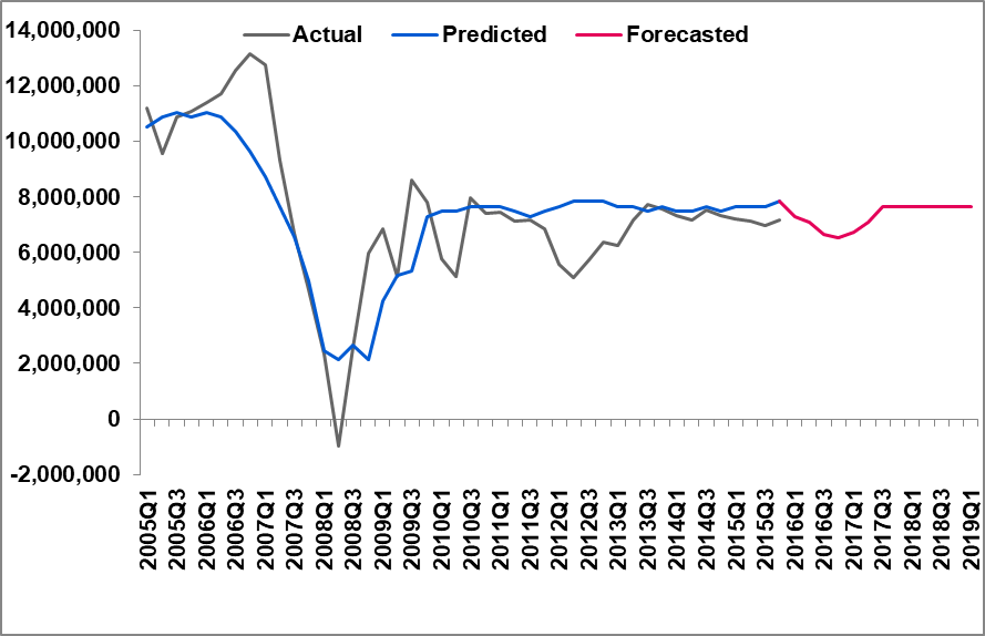
• The projection is done for 13 Quarters 
  • The dip in 2008-2009 is captured well by the model 
  • The severely adverse projection is done for forecasted period 

• Graph
  • Predicted (Blue line) – OLS model 
  • Forecasted (Red line) – ARIMAX model