The bias-variance decomposition is a useful theoretical tool for understanding a learning algorithm‘s performance characteristics. Certain algorithms have a large bias and a low variance by design, and vice versa. Bias-variance is a reducible error, in this article, we will be understanding the concept with ways to decompose the mean squared error. Following are the topics to be covered.
Table of contents
- What is Bias-Variance Decomposition?
- When to use Bias-Variance Decomposition?
- How does this Bias-Variance decomposition work?
As the name suggests there are two important factors to consider: bias and variance. Let’s understand them.
What is Bias-Variance Decomposition?
The bias is defined as the difference between the ML model’s prediction of the values and the correct value. Biasing causes a substantial inaccuracy in both training and testing data. To prevent the problem of underfitting, it is advised that an algorithm be low biased at all times.
Are you looking for a complete repository of Python libraries used in data science, check out here.
The data predicted with high bias is in a straight-line format, which does not fit the data in the data set adequately. Underfitting of data is a term used to describe this type of fitting. This occurs when the theory is overly simplistic or linear in form.
The variance of the model is the variability of model prediction for a particular data point, which tells us about the dispersion of the data. The model with high variance has a very complicated fit to the training data and so is unable to fit correctly on new data.
As a result, while such models perform well on training data, they have large error rates on test data. When a model has a large variance, this is referred to as Overfitting of Data. Variability should be reduced to a minimum while training a data model.

Bias and variance are negatively related, therefore it is essentially difficult to have an ML model with both a low bias and a low variance. When we alter the ML method to better match a specific data set, it results in reduced bias but increases variance. In this manner, the model will fit the data set while increasing the likelihood of incorrect predictions.
The same is true when developing a low variance model with a bigger bias. The model will not fully fit the data set, even though it will lower the probability of erroneous predictions. As a result, there is a delicate balance between biases and variance.

When to use bias-variance decomposition
Since bias and variance are connected to underfitting and overfitting, decomposing the loss into bias and variance helps us understand learning algorithms. Let’s understand certain attributes.
- Low Bias: Tends to suggest fewer implications about the target function’s shape.
- High-Bias: Suggests additional assumptions about the target function’s shape.
- Low Variance: Suggests minor changes to the target function estimate when the training dataset changes.
- High Variance: Suggests that changes to the training dataset cause considerable variations in the target function estimate.
Theoretically, a model should have low bias and low variance but this is impossible to achieve. So, an optimal bias and variance are acceptable. Linear models have low variance but high bias and non-linear models have low bias but high variance.
How does this work?
The total error of a machine learning algorithm has three components: bias, variance and noise. So decomposition is the process of derivation of total error in this case we are taking Mean Squared Error (MSE).
Total error = Bias2 + Variance + Noise
Suppose we have a regression problem where we take in vectors and try to make predictions of a single value. Suppose for the moment that we know the absolute true answer up to an independent random noise. The noise should be independent of any randomness inherent in the vector and should have a mean of zero, so that function is the best possible guess.
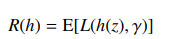
In the above function “R(h)” which is the cost function of the algorithm also known as the risk function. When the risk function is loss it is the squared error. The expected function which is represented by “E” in the above equation contains the random variables. Calculate the average of the probability distributions for hypothesis “h”.
The data x and y are derived from the probability distribution on which the learner will be trained. Since the weights are selected based on the training data, the weights that define h are also obtained from the probability distribution. It can be difficult to determine this distribution, but it does exist. The expectation function consolidates the losses of all potential weight values.
In the above image after doing all the mathematical derivation, we can observe that at last the three components are derived bias, variance and irreducible error or noise.
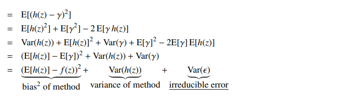
Let’s understand this with an example.

In this example, we’re attempting to match a sine wave with lines, which are obviously not realistic. On the left, we produced 50 distinct lines. The red line in the top right corner represents the anticipated hypothesis which is an average of infinitely many possibilities. The black curve depicts test locations along with the true function.
Because lines do not match sine waves well, we notice that most test points have a substantial bias. Here the bias is the squared difference between the black and red curves.
Some of the test locations, however, exhibit a slight bias, where the sine wave crosses the red line. The variance in the middle represents the predicted squared difference between a random black line and the red line. The irreducible error is the predicted squared difference between a random test point and the sine wave.
Conclusion
We can’t compute the true bias and variance error terms since we don’t know the underlying target function. Nonetheless, bias and variance, as a paradigm, give the tools for understanding the behaviour of machine learning algorithms in their quest for predictive performance. With this article, we have learned the theoretical aspect of decomposition of bias and variance to learn the model performance.