While building most of the supervised machine learning models, the most important task is to devise a function mapping between input and output patterns. There are different mathematical optimization methods used to make this mapping as correct as possible by finding an optimal set of parameters. Gradient descent and stochastic gradient descent are some of these mathematical concepts that are being used for optimization. In this article, we are going to discuss stochastic gradient descent and its implementation from scratch used for a classification porous. The major points to be discussed in the article are listed below.

Table of content 

1. What is gradient descent?
2. Stochastic gradient descent
3. Hands-on Implementation 
   1. Data preparation 
   2. Batch creation and defining functions 
   3. Defining model 
   4. Model testing 

What is gradient descent?

Almost all the machine learning algorithms are based on mathematical operations. Similarly, the gradient descent method in machine learning comes from mathematics where it can be utilised for first-order optimization. It basically works for finding the local minima of any differential function. When talking about the working of the gradient descent we find that it is generated by repeating steps in the opposite direction of the gradient of the function from any point where the gradient is steepest. If the same thing is performed inversely then it can be called a gradient ascent that leads us to a local maximum. we can say that in machine learning, it can be used for optimization that causes improvement in the learning process.

Stochastic gradient descent

Stochastic gradient descent is also a method of optimization. The objective function which needs to be optimised comes with suitable smoothness properties and this suitable smoothness makes the stochastic gradient descent different from the gradient descent. Optimising an objective function with smoothness properties can be considered as the stochastic approximation of gradient descent. This concept is also from mathematics and in machine learning, it can be utilised for minimising the objective function which means finding the local minima of the objective function with suitable smoothness. The smoothness properties can be differentiable or subdifferentiable.

Let’s say there is an optimization function as the following:

In this function, w is a parameter that minimises the function and needs to be estimated. For estimating the w stochastic gradient descent will work on the following steps:

1. Initialization of random w terms
2. Using the w term algorithm will calculate the predictions 
3. Calculate the mean square error between real values and predictions
4. To calculate the updated value of the parameter(w) using the previous value of the parameter and the mean square error.
5. Repeat the calculation of the prediction and updated value of the parameter until the convergence. 

Let’s check how we can implement stochastic gradient descent using python.

Hands-on implementation 

Data preparation 

In this implementation, we will start with importing data. For the trial, we can go with the iris data that can be called from the sklearn library.

from sklearn.datasets import load_iris
data = load_iris()
data.keys()

Output:

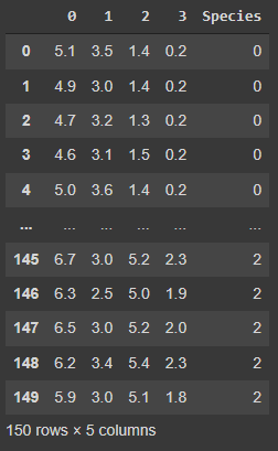
Now we can convert our data into a Pandas data frame using the following lines of codes.

import pandas as pd
dataf = pd.DataFrame(data['data'])
dataf['Species'] = pd.DataFrame(data['target'])
dataf

Output:

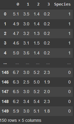
In this article, we will try to optimise the binary classification using stochastic gradient descent and the iris data provides 3 classes in the data set. So in the next, we will convert class second into class 1.

for i in range(len(dataf['Species'])):
    if dataf['Species'][i] == 0:
        dataf['Species'][i] = 1
    else:
        dataf['Species'][i] = 0
dataf

Output:

Let’s split the data.

from sklearn.model_selection import train_test_split
data_feature = dataf.drop(columns = 'Species')
data_class = dataf['Species']
x_train, x_test, y_train, y_test = train_test_split(
    data_feature, data_class, 
    test_size = 0.2,
    random_state = 10
)

After splitting the data we are required to select a few random points of the data to create smoothness.  Before selection, we are required to put target data into train data.

x_train['Species'] = y_train
df = x_train
df       

 Output:

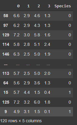
Here we can our final data. Let’s start with the next procedure. 

Batch creation and defining functions 

In this section, we will be defining some functions that are required with the model and we also perform the selection of batches from the data for each iteration. Now we are ready to perform the selection process. We can do that using the following lines of codes 

def stratified_spl(df):
    df1 = df[df['Species'] == 1]
    df0 = df[df['Species'] == 0]
    df1_spl = df1.sample(n=4)
    df0_spl = df0.sample(n=8)
    return pd.concat([df1_spl, df0_spl])

In the above function, we have selected 12 random points for every iteration where 4 data points are collected from class one and 8 data points are collected from the second class.

Using the following lines of codes we can define a sigmoid function 

def sigmoid(X, w):
    z = np.dot(w, X.T)
    return 1/(1+np.exp(-(z)))

Next in the procedure, we are required to separate features and targets from the data with 12 selected random samples. Using the below function we can perform this.

def sep(df):
    df_features = df.drop(columns = 'Species')
    df_label = df['Species']
    df_features['00'] = [1]*12
    return df_features, df_label

Next in the procedure, we will require a function for mean square error. We can define a function for MSE using the following lines of codes.

def SME(X, y, w):
    n = len(X)
    yp = sigmoid(X, w)
    return np.sum((yp-y)**2)/n

After defining the error function, separation, and sigmoid functions, we are ready to make a function for the stochastic gradient descent classifier model.

Defining model 

Now we are ready to make a function for stochastic gradient descent.

def grad_des(df, w, alpha, epoch):
    j = []
    w1 = []
    w1.append(w)
    for i in range(epoch):
        d = stratified_spl(df)
        X, y = sep(d)
        n= len(X)
        yp = sigmoid(X, w)
        
        for i in range(4):
            w[i] -= (alpha/n) * np.sum(-2*X[i]*(y-yp))
        w[4] -= (alpha/n) *np.sum(-2*(y-yp))
        w1.append(list(w))
        j.append(SME(X, y, w))
    return j, w1

Here in the above function, we can see that we are collecting SME and w from each iteration.

Model testing 

Now we are ready to test the model. Let’s define some random numbers as our value of w.

import numpy as np
w = np.random.rand(5)

Now we can use these values and train the dataset with the grad_des function.

j, w1 = grad_des(x_train, w, 0.01, 100)

Here we have calculated the updated weights for the data, now using these we can calculate the mean square error by using the above-defined function.

def err_test(X, y, w):
    er = []
    for i in range(len(w1)):
        er.append(SME(X, y, w[i]))
    return er

Using this function we can calculate the predicted y for each weight and error. Using the following lines of codes we can draw the errors.

import matplotlib.pyplot as plt
def plot(X, y, w):
    error = err_test(X, y, w)
    return plt.scatter(range(len(error)), error)
X = x_train.drop(columns = 'Species')
X['00'] = [1]*len(X)
plot(X, y_train, w1)

Output:

We can also check the errors for the test set by adding some bias.

x_test['00'] = [1]*len(x_test)
plot(x_test, y_test, w1)

Output:

Here we can see that the mean square error is going down with the iterations and it is almost near zero in a few of the last iterations which means our model has worked well.

Final words 

In this article, we have discussed the gradient descent and stochastic gradient descent that is used for optimising the parameters of any function. Along with the discussion we have also gone through an idea that can help us in implementing stochastic gradient descent using python.

References

• Link for the codes