The layer is a collaborative machine learning platform that allows users to create, train, track, and share Machine Learning models. It enables collaboration with semantic versioning, full artefact logging, and dynamic reporting while assisting users in creating production-grade Machine Learning pipelines with a seamless local to cloud transition. This article is focused on building, training and tracking machine learning models with the Layer AI platform. Following are the topics to be covered in this article.

Table of contents

1. Installing Layer
2. Connecting to Layer API
3. Building the model
4. Registering the model to Layer
5. Remote training

In this article, we will build a regression model on a dataset related to the music listed in the top 2000 by Spotify from 2000 to 2019.

Installing Layer

This article uses a Colab notebook so for installing the layer, the syntax would be something like the below.

!pip install layer

Are you looking for a complete repository of Python libraries used in data science, check out here.

Connecting to Layer API

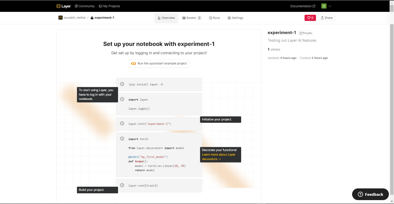
Once the registration is completed on the Layer AI webpage create a project and then connect the notebook to the Layer.

import layer
layer.login()

There is a need for the key to connect the notebook to the API for that just click on the click given by the layer in the output and copy the code to the clipboard and paste it into the output portal.

Once connected to the API initiate the project by using the following code

layer.init("experiment-1")

The Layer will provide a link to the project initiated and all the activities of the current session will be logged in here.

Building the model

Building a regression model for predicting the popularity of the songs based on the different features. For this article using the XG boost algorithm for prediction

Import necessary libraries

import pandas as pd
import numpy as np
import seaborn as sns
import matplotlib.pyplot as plt

Reading and preprocessing the data

data=pd.read_csv('/content/drive/MyDrive/Datasets/songs_normalize.csv')
data[:5]

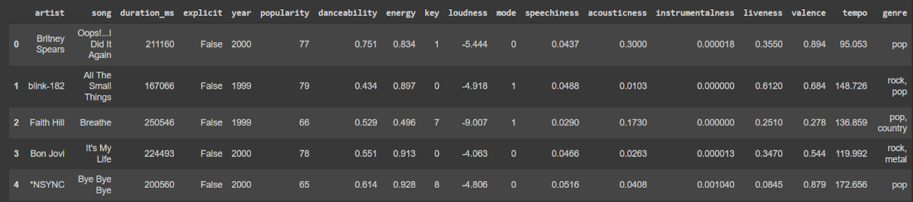
The data used is related to the music industry. It is about the top 2000 songs from 2000 to 2019 according to Spotify. The target column calculates the popularity of the song. Here is a detailed description of the features.

Encoding the categorical variable for processing the data as a training set.

encoder=LabelEncoder()
data['explicit_enc']=encoder.fit_transform(data['explicit'])

X=data.drop(['artist', 'song', 'genre', 'popularity','explicit'],axis=1)
y=data['popularity']

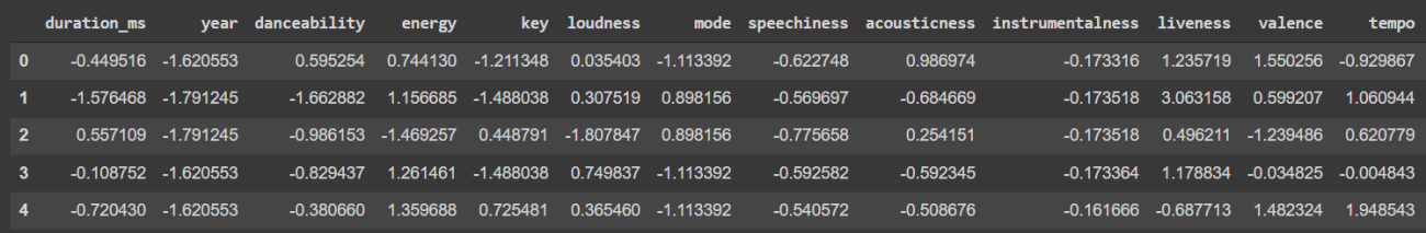
Since there are features related to measurement and measurement has a different unit to measure. So, I need to convert the data into standard form. For this purpose use Standard Scaler from the sklearn library.

std_scale=StandardScaler()
X_scaler=std_scale.fit_transform(X)
X_scaled = pd.DataFrame(X_scaler, columns = X.columns)
X_scaled.head()

Splitting the data into test and train sets using standard division of 30:70 respectively.

X_train, X_test, y_train, y_test = train_test_split(X_scaled, y, test_size=0.30, random_state=42)

Training the model

import xgboost
from sklearn.metrics import mean_squared_error,r2_score

xgb_model = xgboost.XGBRegressor()
xgb_model.fit(X_train, y_train)    
predictions = xgb_model.predict(X_test)
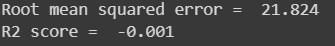
rmse = np.sqrt(mean_squared_error(y_test, predictions))
r_score = r2_score(y_test,predictions)
print("Root mean squared error = ",np.round(rmse,3))
print("R2 score = ",np.round(r_score,3))

Registering the model to Layer

Simply add the decorator “@model” to your training function. The returned trained model will be registered to your Layer Project. To allow experiment tracking, replace “print” with “layer.log.”

@model("experiment_model")
def train_model():
  xgb_model = xgboost.XGBRegressor()
  xgb_model.fit(X_train, y_train)    
  predictions = xgb_model.predict(X_test)
  
  table = pd.DataFrame(zip(predictions,y_test),columns=['Predicted Popularity', "Actual Popularity"])
 
  rmse = np.sqrt(mean_squared_error(y_test, predictions))
  r_score = r2_score(y_test,predictions)
  
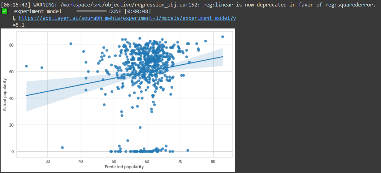
  plt.figure(figsize=(10,6))
  reg_plot=sns.regplot(x=predictions, y=y_test).figure
  plt.xlabel("Predicted popularity")
  plt.ylabel("Actual popularity")
  
  layer.log({"Root mean squared error": rmse})
  layer.log({"R2 score":r_score})
  layer.log({"Regression plot":reg_plot})
  layer.log({"Predictions vs Actual":table[:50]})
  
  return xgb_model
 
xgb_model = train_model()

The decorator “@model” will be used to provide the name of the model so that it can be saved and can be shared or reused in another project. It is necessary to provide all the information related to the model in a function. After completion, a link would be generated where all the track of the model versions and other details would be stored. One can manually visit the same page by ongoing on the model section under the project connected to the notebook.

By using the “log()” all the data is stored in the API server and could be accessed anytime by visiting the models section under the project.

Remote training

The Layer is a sophisticated metadata repository where one can save your models, datasets, and processes. The machine learning pipeline could be registered and executed on Layer in the same way in which it is registered through the notebook. This is particularly beneficial when:

• The training data is too large for the local machine to handle.
• The model needs specialized infrared, like a high-end GPU, which is not available on the local machine.

Instead of executing the train function directly, use “layer.run()” to give it to the Layer. The layer will pickle and execute the function on Layer infra.

layer.run([train_model])

Conclusion

The Layer is a sophisticated metadata repository where you can save your models, datasets, and processes. With this article, we have understood the building, training and registering of an ML model with the Layer AI platform.

References

• Link to the above code
• Documentation of Layer AI