There are a lot of job advertisements on the internet, even on the reputed job advertising sites, which never seem fake. But after the selection, the so-called recruiters start asking for the money and the bank details. Many of the candidates fall in their trap and lose a lot of money and the current job sometimes. So, it is better to identify whether a job advertisement posted on the site is real or fake. Identifying it manually is very difficult and almost impossible. We can apply machine learning to train a model for fake job classification. It can be trained on the previous real and fake job advertisements and it can identify a fake job accurately.

In this article, we will train the machine learning classifier on Employment Scam Aegean Dataset (EMSCAD) to identify the fake job advertisements. First, we will visualize the insights from the fake and real job advertisement and then we will use the Support Vector Classifier in this task which will predict the real and fraudulent class labels for the job advertisements after successful training. Finally, we will evaluate the performance of our classifier using several evaluation metrics. 

The Data Set

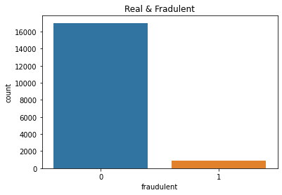
The dataset used in this article is the Employment Scam Aegean Dataset (EMSCAD) dataset which is provided publicly by the University of the Aegean Laboratory of Information & Communication Systems Security. This dataset contains 17,880 real-life job postings in which 17,014 are real and 866 are fake. This dataset is further processed and uploaded on the Kaggle and is available publicly. 

Implementation

First of all, we will implement the required libraries. Make sure to install the libraries before execution such as WordCloud, spacy. 

#Importing Libraries
import re
import string
import numpy as np
import pandas as pd
import random
import matplotlib.pyplot as plt
import seaborn as sns
from sklearn.feature_extraction.text import TfidfVectorizer, CountVectorizer
from sklearn.model_selection import train_test_split
from sklearn.pipeline import Pipeline
from sklearn.base import TransformerMixin
from sklearn.metrics import accuracy_score, plot_confusion_matrix, classification_report, confusion_matrix
from wordcloud import WordCloud
import spacy
from spacy.lang.en.stop_words import STOP_WORDS
from spacy.lang.en import English
from sklearn.svm import SVC

After importing the required libraries, we will read the data set to the program.

#Reading dataset
data = pd.read_csv('fake_job_postings.csv')

#We will check the shape of the dataset and the top five elements of the dataset.

#Shape of the dataset
data.shape




#Head of the dataset
data.head()

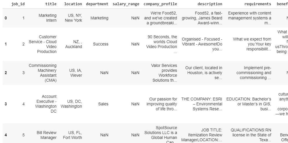
In the head of the dataset, we can see that missing values are present as NaN. We will check all the missing values in the replace them with blank.

data.interpolate(inplace=True)
data.isnull().sum()





















#Delete the unnecessary columns
columns=['job_id', 'telecommuting', 'has_company_logo', 'has_questions', 'salary_range', 'employment_type']
for col in columns:
    del data[col]

#Fill NaN values with blank space
data.fillna(' ', inplace=True)

data.head()

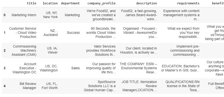
The data set is now free from the missing values. Now, we will check the total number of fraudulent postings and real postings.

#Fraud and Real visualization
sns.countplot(data.fraudulent).set_title('Real & Fradulent')
data.groupby('fraudulent').count()['title'].reset_index().sort_values(by='title',ascending=False)

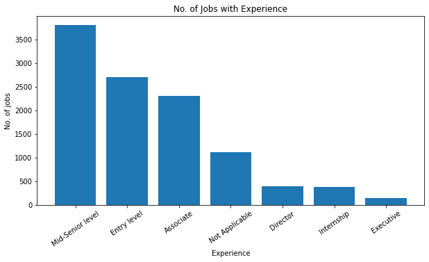
In the next step, we will visualize the number of job postings by countries and by experience. 

#Visualize job postings by countries
def split(location):
    l = location.split(',')
    return l[0]

data['country'] = data.location.apply(split)

country = dict(data.country.value_counts()[:11])
del country[' ']
plt.figure(figsize=(8,6))
plt.title('Country-wise Job Posting', size=20)
plt.bar(country.keys(), country.values())
plt.ylabel('No. of jobs', size=10)
plt.xlabel('Countries', size=10)
























#Visualize the required experiences in the jobs
experience = dict(data.required_experience.value_counts())
del experience[' ']
plt.figure(figsize=(10,5))
plt.bar(experience.keys(), experience.values())
plt.title('No. of Jobs with Experience')
plt.xlabel('Experience', size=10)
plt.ylabel('No. of jobs', size=10)
plt.xticks(rotation=35)
plt.show()

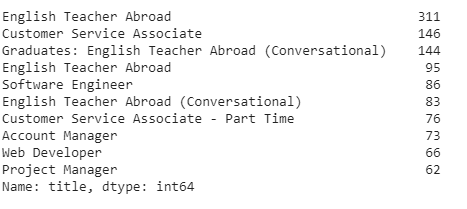
Here, we will check the count of titles in all job postings, in fraudulent job postings and in real job postings.

#Most frequent jobs
print(data.title.value_counts()[:10])














#Titles and count of fraudulent jobs
print(data[data.fraudulent==1].title.value_counts()[:10])













#Titles and count of real jobs
print(data[data.fraudulent==0].title.value_counts()[:10])

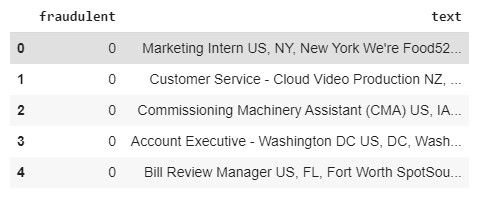
In the next step, the dataset will be preprocessed for training. For this purpose, all the important text data is combined in one column and rest are deleted except the target column.

#combine text in a single column to start cleaning our data
data['text']=data['title']+' '+data['location']+' '+data['company_profile']+' '+data['description']+' '+data['requirements']+' '+data['benefits']
del data['title']
del data['location']
del data['department']
del data['company_profile']
del data['description']
del data['requirements']
del data['benefits']
del data['required_experience']
del data['required_education']
del data['industry']
del data['function']
del data['country']

data.head()

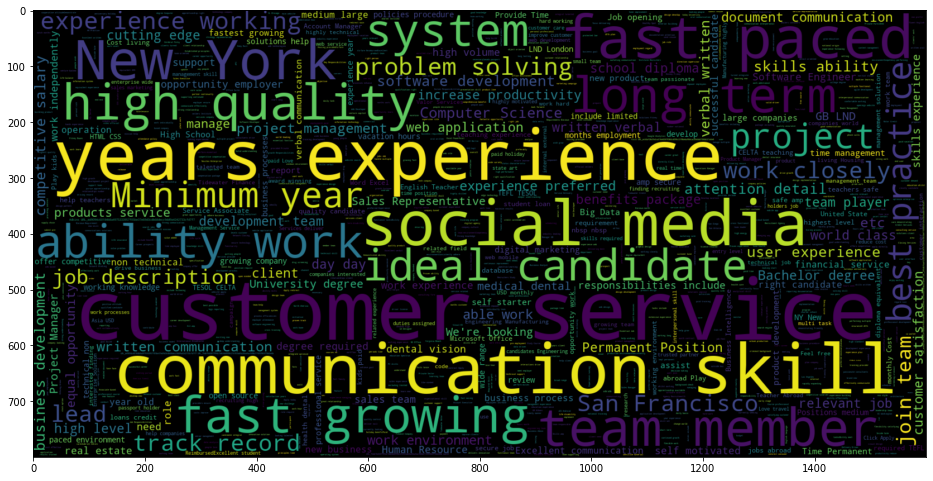
To visualize the fraud and real job postings, the WordCloud is used to see the top occurring keywords in the data. To do so, fraud and real job postings are separated into two text files and WordCloud has plotted accordingly. 

#Separate fraud and actual jobs
fraudjobs_text = data[data.fraudulent==1].text
actualjobs_text = data[data.fraudulent==0].text

#Fraudulent jobs word cloud
STOPWORDS = spacy.lang.en.stop_words.STOP_WORDS
plt.figure(figsize = (16,14))
wc = WordCloud(min_font_size = 3,  max_words = 3000 , width = 1600 , height = 800 , stopwords = STOPWORDS).generate(str(" ".join(fraudjobs_text)))
plt.imshow(wc,interpolation = 'bilinear')






















#Actual jobs wordcloud
plt.figure(figsize = (16,14))
wc = WordCloud(min_font_size = 3,  max_words = 3000 , width = 1600 , height = 800 , stopwords = STOPWORDS).generate(str(" ".join(actualjobs_text)))
plt.imshow(wc,interpolation = 'bilinear')

The dataset is cleaned and preprocessed using the below lines of codes.

#Cleaning and preprocessing
# Create our list of punctuation marks
punctuations = string.punctuation

# Create our list of stopwords
nlp = spacy.load('en')
stop_words = spacy.lang.en.stop_words.STOP_WORDS

# Load English tokenizer, tagger, parser, NER and word vectors
parser = English()

# Creating our tokenizer function
def spacy_tokenizer(sentence):
    # Creating our token object, which is used to create documents with linguistic annotations.
    mytokens = parser(sentence)

    # Lemmatizing each token and converting each token into lowercase
    mytokens = [ word.lemma_.lower().strip() if word.lemma_ != "-PRON-" else word.lower_ for word in mytokens ]

    # Removing stop words
    mytokens = [ word for word in mytokens if word not in stop_words and word not in punctuations ]

    # return a preprocessed list of tokens
    return mytokens

# Custom transformer using spaCy
class predictors(TransformerMixin):
    def transform(self, X, **transform_params):
        # Cleaning Text
        return [clean_text(text) for text in X]

    def fit(self, X, y=None, **fit_params):
        return self

    def get_params(self, deep=True):
        return {}

# Basic function to clean the text
def clean_text(text):
    # Removing spaces and converting text into lowercase
    return text.strip().lower()

# Splitting dataset in train and test
X_train, X_test, y_train, y_test = train_test_split(data.text, data.fraudulent, test_size=0.3)

#Train-test shape
print(X_train.shape)
print(y_train.shape)
print(X_test.shape)
print(y_test.shape)

Once we are ready with the training and test data, we will train the machine learning model to classify the fraudulent and real job postings. In this task, we will use the Support Vector Classifier. The Pipeline is used to bind the cleaning, vectorization and classification works together.

#Support Vector Machine Classifier
# Create pipeline using Bag of Words
pipe = Pipeline([("cleaner", predictors()),
                 ('vectorizer', CountVectorizer(tokenizer = spacy_tokenizer, ngram_range=(1,3))),
                 ('classifier', SVC())])

#Training the model.
pipe.fit(X_train,y_train)

Fake Job Classification

After successful training of the classifier, we will make predictions through it on the test data and obtain the accuracies by evaluation metrics. 

# Predicting with a test dataset
y_pred = pipe.predict(X_test)

# Model Accuracy
print("Classification Accuracy:", accuracy_score(y_test, y_pred))
print("Classification Report\n")
print(classification_report(y_test, y_pred))
print("Confusion Matrix\n")
print(confusion_matrix(y_test, y_pred))



















fig, ax = plt.subplots(figsize=(10, 10))
plot_confusion_matrix(pipe, X_test, y_test, values_format=' ', ax=ax) 
plt.title('Confusion Matrix')
plt.show()

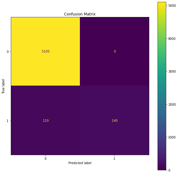
So, we can see that the Support Vector Classifier has given the accuracy score of 97.78% and for 5354 test observations, it has correctly predicted the class labels for 5245 job postings.