With the rapid development of mobile devices, speech-related technology is booming like never before. Many service providers like Google offer the ability to search through the voice on the android platform. In contrast, on the other hand, the personnel assistance Microsoft’s ‘Cortana’, Apple’s ‘Siri’ and Amazon’s ‘Alexa’ are using a utility like keyword recognition to interact with the system. For android mobile phones, ‘Ok Google’ uses this functionality to search a particular keyword to initiate the voice-based commands. Keyword recognition refers to speech technology that recognizes the existence of a word or short phrase within a given stream of audio. It is synonymously referred to as keyword spotting.
The actual environment of Keyword recognition is quite more complex than this demonstration. This article focuses on knowing the basic idea used behind the keyword recognition for short audio files of one second. As the convolutional networks outperform when it comes to image-based classification tasks, we are leveraging this behaviour of convolutional neural networks to the keyword recognition/classification task. For that, we are converting our audio files to spectrogram nothing but the visual representation of audio files so that we can use convolutional neural networks. Before proceeding to the coding, we look at the details of the spectrogram and its features.
What is a spectrogram?
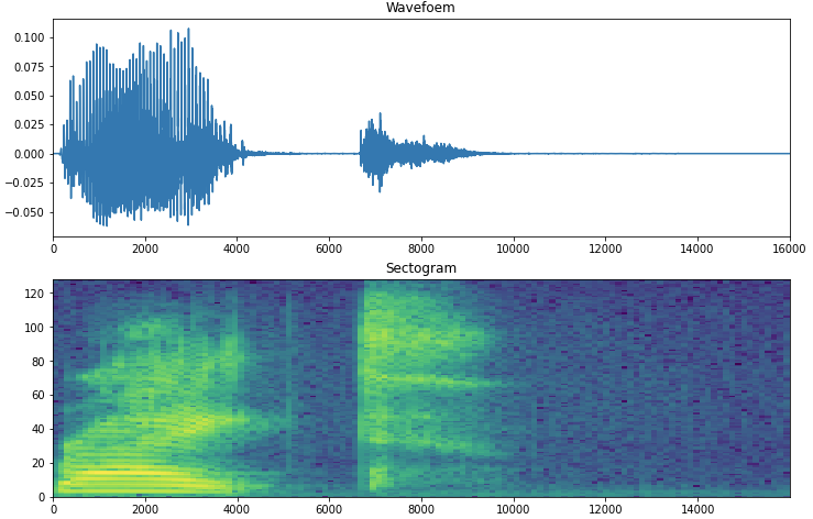
A spectrogram is a detailed view of audio that represents time, frequency, and amplitude in one graph. A spectrogram can visually reveal broadband, electrical or intermittent noise in the audio, allowing you to isolate those audio problems by just citing the graph. We can read a spectrogram like; it keeps time on the X-axis and places frequency on the Y-axis, and the aptitude of the signal is represented as a sort of heat map or scale of color saturation. It was originally produced as black and white diagrams on paper by a sound spectrograph device, but nowadays, these graphs are created by software and can be any range of color.
Spectrograms map out sounds similar to a musical score; the difference is that it maps frequency instead of musical notes. Seeing frequency energy distribution over time allows us to distinguish each sound element and its harmonic structures clearly. This is especially useful in acoustic studies when analysing sounds such as bird songs or musical instruments. The graph does not look cool, but it tells you a lot of information about the audio file even without listening to it.
As we know how CNN is good at unstructured data such as images, we will use a CNN-based model to classify some keywords. The below implementation shows you how to convert the audio files to that of spectrogram and CNN model, which classify the keywords. The following code is in reference to the official implementation.
Import all dependencies:
 import matplotlib.pyplot as plt
 import numpy as np
 import seaborn as sns
 import tensorflow as tf
 from tensorflow.keras.layers.experimental import preprocessing
 from tensorflow.keras import layers
 from tensorflow.keras import models
 from IPython import display
 from sklearn.metrics import classification_report
 import pathlib
 import os
 seed = 42
 tf.random.set_seed(seed)
 np.random.seed(seed)
Load data and train test split:
The below code is used to import the Speech Command Dataset, which contains nearly 105000 WAV files of 30 different keywords. Although the original dataset nearly weighs around 8GB, we use a small portion of this dataset to save memory and time. The minimized dataset contains keywords as “down, go, left, right, no, stop, up and yes”.
 data_dir = pathlib.Path('data/mini_speech_commands')
 if not data_dir.exists():
   tf.keras.utils.get_file('mini_speech_commands.zip',
       origin="http://storage.googleapis.com/download.tensorflow.org/data/mini_speech_commands.zip",
       extract=True,cache_dir='.', cache_subdir='data')
 labels = np.array(tf.io.gfile.listdir(str(data_dir)))
 labels = labels[labels != 'README.md']
 print('Commands',labels)
Output:
Commands ['no' 'right' 'stop' 'go' 'down' 'up' 'yes' 'left']
Extract the audio files into list;
 files = tf.io.gfile.glob(str(data_dir)+'/*/*')
 files = tf.random.shuffle(files)
 num_samples = len(files)
 print("number of total samples: ",num_samples)
 print("examples per labels: ",len(tf.io.gfile.listdir(str(data_dir/labels[0]))))
 print("file tensor: ",files[0])

Train_test split;
 train = files[:6400]
 vali = files[6400:6400+800]
 test = files[-800:]
Reading audio files and labels:
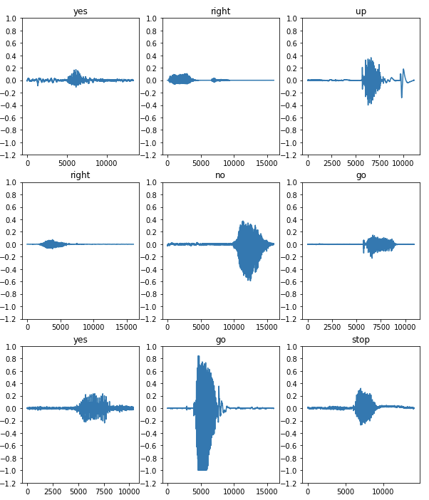
The files will initially be read as binary files, which we later need to convert into tensors. WAV file contains time series data with a set of numbers of samples per second. Each sample represents the amplitude of the audio signal at a specific time. tf.audio.decode_wav is used which will return WAV encoded audio as tensor.
 ## binary file will be converted into numerical tensors
 def audio_decode(audio_binary):
   audios,_ = tf.audio.decode_wav(audio_binary)
   return tf.squeeze(audios,axis=-1)
 ## labels for each wave file
 def get_label_(file_path):
   part = tf.strings.split(file_path, os.path.sep)
   return part[-2]
 ## create supevised training method which takes audio file along with label
 def waveform_and_label(file_path):
   labels = get_label_(file_path)
   audio_binary = tf.io.read_file(file_path)
   waveforms = audio_decode(audio_binary)
   return waveforms,labels
 # apply the Process_path to build training set to extract audio-label pairs
 # and check the result
 AUTOTUNE = tf.data.AUTOTUNE
 files_data = tf.data.Dataset.from_tensor_slices(train)
 waveform_data = files_ds.map(waveform_and_label, num_parallel_calls = AUTOTUNE)
Visualise the waveform with its labels:
 row = 3
 col = 3
 n = row*col
 fig, axes = plt.subplots(row,col, figsize=(10,12))
 for i,(audios,labels) in enumerate(waveform_data.take(n)):
   r1 = i// col
   c1 = i % col
   axs = axes[r1][c1]
   axs.plot(audios.numpy())
   axs.set_yticks(np.arange(-1.2,1.2,0.2))
   labels = labels.numpy().decode('utf-8')
   axs.set_title(labels)
 plt.show()
Create a function that will return spectrogram:
We convert waveform into spectrograms by applying the short-time Fourier transform (STFT) to convert audio into the time-frequency domain. The STFT by using tf.signal.stft splits the signal into a window of time and runs a Fourier transform on each window that returns a 2-D tensor to apply the convolutional layers. STFT produces an array representing phase and amplitude information, but we will be using only amplitude information for model building for that tf.abs used to derive it.
Choose frame_lenght and frame_step precisely so that the output image will be nearly square. We will also be using zero paddings so that all files will be equal in length.
 def get_spectogram(waveforms):
   ## padding the files with less than 1600 samples
   padding = tf.zeros([16000] - tf.shape(waveforms),dtype=tf.float32)
   ## concate audio with padding for equal lenght
   waveforms = tf.cast(waveforms, tf.float32)
   equal_lenght = tf.concat([waveforms,padding], 0)
   spectogram = tf.signal.stft(equal_lenght,frame_length=255,frame_step=128)
   spectogram = tf.abs(spectogram)
   return spectogram
Compare the waveform, spectrogram and audio file of one sample;
 for waveforms,labels in waveform_data.take(2):
   labels = labels.numpy().decode('utf-8')
   spectogram = get_spectogram(waveforms)
 print('label:',labels)
 print('waveform shape:',waveforms.shape)
 print('Spectogram shape:',spectogram.shape)
 print('Audio playback')
 display.display(display.Audio(waveforms, rate=16000))

Audio file:
Plot the spectrogram of one sample;
 def plot_spectogram(spectogram, axs):
   # convert frequencies into log scale so that time represented on
   # x-axis
   log_scale = np.log(spectogram.T)
   height = log_scale.shape[0]
   width = log_scale.shape[1]
   x = np.linspace(0, np.size(spectogram),num=width, dtype=int)
   y = range(height)
   axs.pcolormesh(x,y, log_scale)
 fig,axes = plt.subplots(2,figsize=(12,8))
 time_scale = np.arange(waveforms.shape[0])
 axes[0].plot(time_scale, waveforms.numpy())
 axes[0].set_title('Wavefoem')
 axes[0].set_xlim([0,16000])
 plot_spectogram(spectogram.numpy(),axes[1])
 axes[1].set_title('Sectogram')
 plt.show()
Transform the waveform dataset in spectrogram dataset with corresponding labels and visualise the spectrograms;
 def spectogram_and_label(audios,label):
   spectogram = get_spectogram(audios)
   spectogram = tf.expand_dims(spectogram,-1)
   labels_id = tf.argmax(label == lables)
   return spectogram, labels_id
spectogram_data = waveform_data.map(spectogram_and_label,num_parallel_calls=AUTOTUNE)
 row = 3
 col = 3
 n = row*col
 fig, axes = plt.subplots(row,col, figsize=(10,12))
 for i,(spectogram,label_id) in enumerate(spectogram_data.take(n)):
   r2 = i// col
   c2 = i % col
   axs = axes[r2][c2]
   plot_spectogram(np.squeeze(spectogram.numpy()),axs)
   axs.set_title(commands[label_id.numpy()])
   axs.axis('off')
 plt.show()

Run the preprocessing step on test and validation set:
 def create_dataset(files):
   files_data = tf.data.Dataset.from_tensor_slices(files)
   output_data = files_data.map(waveform_and_label,num_parallel_calls=AUTOTUNE)
   output_data = output_ds.map(spectogram_and_label,num_parallel_calls = AUTOTUNE)
   return output_data
 train_data = spectogram_ds
 vali_data = create_dataset(vali)
 test_data = create_dataset(test)
Build the model:
Batch the dataset and add cache() and prefetch() operation to reduce latency;
 batch_size = 64
 train_data = train_data.batch(batch_size)
 vali_data = vali_data.batch(batch_size)
 train_data = train_data.cache().prefetch(AUTOTUNE)
 vali_data = vali_data.cache().prefetch(AUTOTUNE)
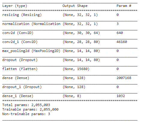
Along with CNN layers, the model is also having preprocessing layers such as resizing and normalisation;
 for spectogram, _ in spectogram_data.take(1):
   input_shape1 = spectogram.shape
 print("input shape:",input_shape1)
 num_labels = len(labels)
 norma_layer = preprocessing.Normalization()
 norma_layer.adapt(spectogram_data.map(lambda x,_: x))
 model = models.Sequential([
         layers.Input(shape=input_shape1),
         preprocessing.Resizing(32,32),
         norma_layer,
         layers.Conv2D(64,3, activation='relu'),
         layers.Conv2D(80,3,activation='relu'),
         layers.MaxPooling2D(),
         layers.Dropout(0.25),
         layers.Flatten(),
         layers.Dense(128,activation='relu'),
         layers.Dropout(0.5),
         layers.Dense(num_labels)
 ])
model.summary()
model.compile(loss=tf.keras.losses.SparseCategoricalCrossentropy(from_logits=True),optimizer='adam',metrics=['accuracy'])
 history = model.fit(train_ds,validation_data=vali_ds,epochs=10,
        callbacks = tf.keras.callbacks.EarlyStopping(verbose=1,patience=2))

Evaluate the model:
 test_audios = []
 test_labels = []
 for audios,labels in test_ds:
   test_audios.append(audios.numpy())
   test_labels.append(labels.numpy())
 test_audios = np.array(test_audios)
 test_labels = np.array(test_labels)
 y_predi = np.argmax(model.predict(test_audios),axis=1)
 y_true = test_labels
 test_accuracy = sum(y_predi == y_true) / len(y_true)
 print('Test accuracy:',test_accuracy)
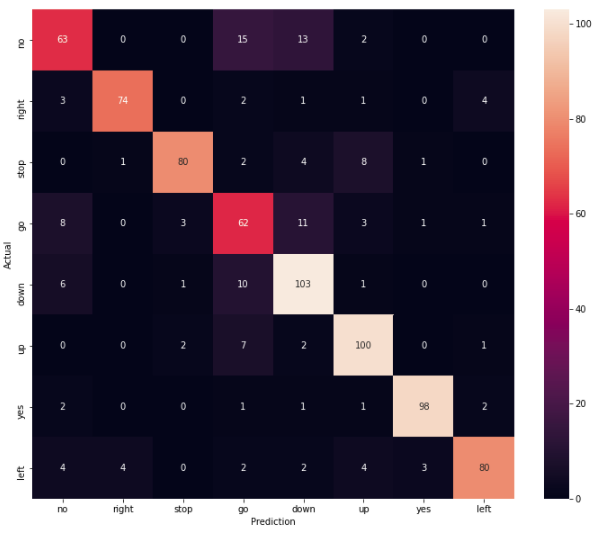
Test accuracy is around 83%
Plot confusion matrix and classification report;
 print(classification_report(y_true,y_pred,))
 confusion_mat = tf.math.confusion_matrix(y_true,y_predi)
 plt.figure(figsize=(12,10))
 sns.heatmap(confusion_mat,xticklabels=commands,yticklabels=commands,annot=True,fmt='g')
 plt.xlabel('Prediction')
 plt.ylabel('Actual')
 plt.show()

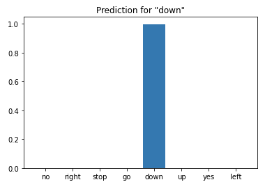
Infer the model on audio file;
 sample_file = '/content/data/mini_speech_commands/down/004ae714_nohash_0.wav'
 sample_data = create_dataset([str(sample_file)])
 for spectogram, label in sample_ds.batch(1):
   prediction = model(spectogram)
   plt.bar(labels, tf.nn.softmax(prediction[0]))
   plt.title(f'Prediction for "{labels[label[0]]}"')
   plt.show()
Conclusion
This is all about keyword recognition using simple convolutional neural networks where we have used 1-second audio files saying eight different words. This was the basic idea of how keyword recognition works where the actual system is a bit complex. Coming towards the model’s performance for a given audio file, the model predicts the file as down perfectly. Precision for the words ‘no’ and ‘go’ is poor. This might be due to imbalance because we have not sampled the data uniformly for all classes. For the rest of the classes, parameters are acceptable.


