


With the successful implementation of deep learning models in a variety of applications, now it is the time to get results not only accurate but with a faster speed. To get much accurate results, the size of data definitely matters, but when this size impacts the training time of machine learning models, it is always a concern. To overcome this issue of training time, the TPU runtime environment is used to accelerate the same. In this order, PyTorch has been supporting the machine learning implementation by providing cutting-edge hardware accelerators. The PyTorch support for Cloud TPUs is achieved via integration with XLA (Accelerated Linear Algebra), a compiler for linear algebra that can target multiple types of hardware, including CPU, GPU, and TPU.
This article demonstrates how we can implement a Deep Learning model using PyTorch with TPU to accelerate the training process. Here, we define a Convolutional Neural Network (CNN) model using PyTorch and train this model in the PyTorch/XLA environment. XLA connects the CNN model with the Google Cloud TPU (Tensor Processing Unit) in the distributed multiprocessing environment. In this implementation, 8 TPU cores are used to create a multiprocessing environment. We will test this PyTorch deep learning framework in Fashion MNIST classification and observe the training time and accuracy.
Implementing CNN Using PyTorch With TPU
We will implement the execution in Google Colab because it provides free of cost cloud TPU (Tensor Processing Unit). Before proceeding further, in the Colab notebook, go to ‘Edit’ and then ‘Notebook Settings’ and select the ‘TPU’ as the ‘Hardware accelerator’ from the list as given in the below screenshot.

To verify whether the TPU environment is working properly, run the below line of codes.
import os
assert os.environ['COLAB_TPU_ADDR']
It will be executed successfully if the TPU is enabled otherwise it will return the ‘KeyError: ‘COLAB_TPU_ADDR’’. You can also check the TPU by printing its address.
TPU_Path = 'grpc://'+os.environ['COLAB_TPU_ADDR']
print('TPU Address:', TPU_Path)
After enabling the TPU, we will install the compatible wheels and dependencies to setup the XLA environment using the below code.
VERSION = "20200516"
!curl https://raw.githubusercontent.com/pytorch/xla/master/contrib/scripts/env-setup.py -o pytorch-xla-env-setup.py
!python pytorch-xla-env-setup.py --version $VERSION
Once it is installed successfully, we will proceed to define the methods for loading the data set, initializing the CNN model, training and testing. First of all, we will import the required libraries.
import numpy as np
import os
import time
import torch
import torch.nn as nn
import torch.nn.functional as F
import torch.optim as optim
import torch_xla
import torch_xla.core.xla_model as xm
import torch_xla.debug.metrics as met
import torch_xla.distributed.parallel_loader as pl
import torch_xla.distributed.xla_multiprocessing as xmp
import torch_xla.utils.utils as xu
from torchvision import datasets, transforms
After that, we will define the hyperparameters to be required further.
# Define Parameters
FLAGS = {}
FLAGS['datadir'] = "/tmp/mnist"
FLAGS['batch_size'] = 128
FLAGS['num_workers'] = 4
FLAGS['learning_rate'] = 0.01
FLAGS['momentum'] = 0.5
FLAGS['num_epochs'] = 50
FLAGS['num_cores'] = 8
FLAGS['log_steps'] = 20
FLAGS['metrics_debug'] = False
The below code snippet will define the CNN model as a PyTorch instance and the functions for loading the data, training the model and testing the model.
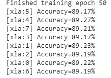
SERIAL_EXEC = xmp.MpSerialExecutor()

class FashionMNIST(nn.Module):

  def __init__(self):
    super(FashionMNIST, self).__init__()
    self.conv1 = nn.Conv2d(1, 10, kernel_size=5)
    self.bn1 = nn.BatchNorm2d(10)
    self.conv2 = nn.Conv2d(10, 20, kernel_size=5)
    self.bn2 = nn.BatchNorm2d(20)
    self.fc1 = nn.Linear(320, 50)
    self.fc2 = nn.Linear(50, 10)

  def forward(self, x):
    x = F.relu(F.max_pool2d(self.conv1(x), 2))
    x = self.bn1(x)
    x = F.relu(F.max_pool2d(self.conv2(x), 2))
    x = self.bn2(x)
    x = torch.flatten(x, 1)
    x = F.relu(self.fc1(x))
    x = self.fc2(x)
    return F.log_softmax(x, dim=1)

# Only instantiate model weights once in memory.
WRAPPED_MODEL = xmp.MpModelWrapper(FashionMNIST())

def train_mnist():
  torch.manual_seed(1)

  def get_dataset():
    norm = transforms.Normalize((0.1307,), (0.3081,))
    train_dataset = datasets.FashionMNIST(
        FLAGS['datadir'],
        train=True,
        download=True,
        transform=transforms.Compose(
            [transforms.ToTensor(), norm]))
    test_dataset = datasets.FashionMNIST(
        FLAGS['datadir'],
        train=False,
        download=True,
        transform=transforms.Compose(
            [transforms.ToTensor(), norm]))


    return train_dataset, test_dataset


  # Using the serial executor avoids multiple processes to
  # download the same data.
  train_dataset, test_dataset = SERIAL_EXEC.run(get_dataset)

  train_sampler = torch.utils.data.distributed.DistributedSampler(
    train_dataset,
    num_replicas=xm.xrt_world_size(),
    rank=xm.get_ordinal(),
    shuffle=True)

  train_loader = torch.utils.data.DataLoader(
      train_dataset,
      batch_size=FLAGS['batch_size'],
      sampler=train_sampler,
      num_workers=FLAGS['num_workers'],
      drop_last=True)

  test_loader = torch.utils.data.DataLoader(
      test_dataset,
      batch_size=FLAGS['batch_size'],
      shuffle=False,
      num_workers=FLAGS['num_workers'],
      drop_last=True)

  # Scale learning rate to world size
  lr = FLAGS['learning_rate'] * xm.xrt_world_size()

  # Get loss function, optimizer, and model
  device = xm.xla_device()
  model = WRAPPED_MODEL.to(device)
  optimizer = optim.SGD(model.parameters(), lr=lr, momentum=FLAGS['momentum'])
  loss_fn = nn.NLLLoss()

  def train_fun(loader):
    tracker = xm.RateTracker()
    model.train()
    for x, (data, target) in enumerate(loader):
      optimizer.zero_grad()
      output = model(data)
      loss = loss_fn(output, target)
      loss.backward()
      xm.optimizer_step(optimizer)
      tracker.add(FLAGS['batch_size'])
      if x % FLAGS['log_steps'] == 0:
        print('[xla:{}]({}) Loss={:.5f}'.format(
            xm.get_ordinal(), x, loss.item(), time.asctime()), flush=True)

  def test_fun(loader):
    total_samples = 0
    correct = 0
    model.eval()
    data, pred, target = None, None, None
    for data, target in loader:
      output = model(data)
      pred = output.max(1, keepdim=True)[1]
      correct += pred.eq(target.view_as(pred)).sum().item()
      total_samples += data.size()[0]

    accuracy = 100.0 * correct / total_samples
    print('[xla:{}] Accuracy={:.2f}%'.format(
        xm.get_ordinal(), accuracy), flush=True)
    return accuracy, data, pred, target

  # Train and eval loops
  accuracy = 0.0
  data, pred, target = None, None, None
  for epoch in range(1, FLAGS['num_epochs'] + 1):
    para_loader = pl.ParallelLoader(train_loader, [device])
    train_fun(para_loader.per_device_loader(device))
    xm.master_print("Finished training epoch {}".format(epoch))

    para_loader = pl.ParallelLoader(test_loader, [device])
    accuracy, data, pred, target  = test_fun(para_loader.per_device_loader(device))
    if FLAGS['metrics_debug']:
      xm.master_print(met.metrics_report(), flush=True)

  return accuracy, data, pred, target
Now, to plot the results as the predicted label and actual labels for the test images, the below function module will be used.
# Result Visualization
import math
from matplotlib import pyplot as plt

M, N = 5, 5
RESULT_IMG_PATH = '/tmp/test_result.png'

def plot_results(images, labels, preds):
  images, labels, preds = images[:M*N], labels[:M*N], preds[:M*N]
  inv_norm = transforms.Normalize((-0.1307/0.3081,), (1/0.3081,))

  num_images = images.shape[0]
  fig, axes = plt.subplots(M, N, figsize=(12, 12))
  fig.suptitle('Predicted Lables')

  for i, ax in enumerate(fig.axes):
    ax.axis('off')
    if i >= num_images:
      continue
    img, label, prediction = images[i], labels[i], preds[i]
    img = inv_norm(img)
    img = img.squeeze() # [1,Y,X] -> [Y,X]
    label, prediction = label.item(), prediction.item()
    if label == prediction:
      ax.set_title(u'Actual {}/ Predicted {}'.format(label, prediction), color='blue')
    else:
      ax.set_title(
          'Actual {}/ Predicted {}'.format(label, prediction), color='red')
    ax.imshow(img)
  plt.savefig(RESULT_IMG_PATH, transparent=True)
Now, we are all set to train the model on the Fashion MNIST dataset. Before starting the training, we will record the start time and after finishing the training, we will record the end time and print the total training time for 50 epochs.
# Start training processes def train_cnn(rank, flags): global FLAGS FLAGS = flags torch.set_default_tensor_type('torch.FloatTensor') accuracy, data, pred, target = train_mnist() if rank == 0: # Retrieve tensors that are on TPU core 0 and plot. plot_results(data.cpu(), pred.cpu(), target.cpu()) xmp.spawn(train_cnn, args=(FLAGS,), nprocs=FLAGS['num_cores'], start_method='fork')...
Once the training ends successfully, we will print the total time taken during the training.
end_time = time.time()
print('Total Training time = ',end_time-start_time )
![]()
As we can see above, this approach has taken 269 seconds or about 4.5 minutes that means less than 5 minutes to train the PyTorch model in 50 epochs. Finally, we will visualize the predictions by the trained model.
from google.colab.patches import cv2_imshow
import cv2
img = cv2.imread(RESULT_IMG_PATH, cv2.IMREAD_UNCHANGED)
cv2_imshow(img)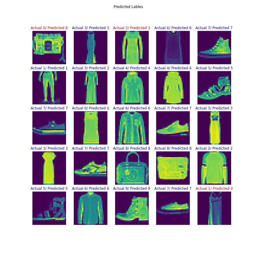
So, we can conclude that using the TPU to implement a deep learning model results in fast training as we have seen above. The training of the CNN model on 40,000 training images in 50 epochs has been performed in less than 5 minutes. We have also obtained more than 89% accuracy during the training. So training the deep learning models on TPU is always a benefit in terms of time and accuracy.
References:-
- Joe Spisak, “Get started with PyTorch, Cloud TPUs, and Colab”.
- “PyTorch on XLA Devices”, PyTorch release.
- “Training PyTorch models on Cloud TPU Pods”, Google Cloud Guides.