Pretrained models in machine learning is the process of saving the models in a pickle or joblib format and using them to make predictions for the data it is trained for. Saving the models in the pipeline facilitates the interpretation of model coefficients and taking up predictions from the saved model weights and parameters during model deployment for production. So this article provides a brief overview of how to implement a random forest classifier model and save it in a pickle format and use the pretrained model for predictions during production.

Table of Contents

1. An introduction to pre-trained models 
2. Building a classification model from scratch
3. Saving the model in pickle format
4. Loading the saved model
5. Obtaining predictions from the loaded model
6. Summary

An introduction to pre-trained models

Pretrained models are the models obtained after maturing through various processes of a typical machine learning model lifecycle. Pretrained models are the models developed to obtain predictions for problems of similar kinds and help us to save huge training time. So for similar kinds of data, the pretrained models can be loaded at the start and later modified as required or the same model which is pretrained for similar kinds of features can be used to obtain predictions.

Note:-

Pretrained models may always not be accurate and may be biased to similar kinds of features in data. So in general it is advisable to understand if the pretrained models are biased towards any particular features before using them.

Building a random forest classification model from scratch

Here we have used a health-care dataset to build a random forest classification model from scratch and also the required preprocessing steps to adhere are shown below. So now let’s look into the steps involved in building a random forest classification model.

Are you looking for a complete repository of Python libraries used in data science, check out here.

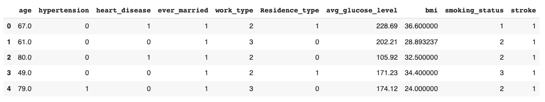
So first let us visualize the top 5 entries of the dataset.

Data Preprocessing

So the above dataset was checked for null values and the corresponding features of null values were appropriately imputed for correct values. So from the dataset id and gender features were removed as they seemed to be less significant and did not possess any important information. 

df=df.drop(['id','gender'],axis=1)

So now the categorical features of the dataset were encoded to numerical features using the LabelEncoder of the scikit module as shown below.

from sklearn.preprocessing import LabelEncoder
le=LabelEncoder() ## creating a label encoder instance for fitting
df['ever_married']=le.fit_transform(df['ever_married'])
df['work_type']=le.fit_transform(df['work_type'])
df['Residence_type']=le.fit_transform(df['Residence_type'])
df['smoking_status']=le.fit_transform(df['smoking_status'])

So once the encoding was complete the dataset was again visualized to understand how LabelEncoder has encoded the categorical features present in the data.

Now as we have appropriate preprocessed data let’s proceed ahead with splitting the data.

Splitting the data

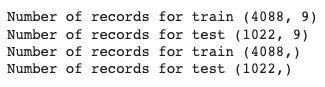
The preprocessed data is now being split using the scikit learn module as shown below along with validating the number of records for training and testing the model.

from sklearn.model_selection import train_test_split
X_train,X_test,Y_train,Y_test=train_test_split(X,y,test_size=0.2,random_state=42)
print('Number of records for train',X_train.shape)
print('Number of records for test',X_test.shape)
print('Number of records for train',Y_train.shape)
print('Number of records for test',Y_test.shape)

Implementing the random forest model

Using the split data a random forest classifier model was implemented as shown below along with evaluating various parameters like accuracy score and Area Under Curve (AUC) to determine model performance and validate any signs of overfitting. 

The steps involved in implementing a random forest model and evaluating the parameters are shown below.

from sklearn.ensemble import RandomForestClassifier
rfc_class=RandomForestClassifier(random_state=42)
rfc_base=rfc_class.fit(X_train,Y_train)
rfc_pred=rfc_base.predict(X_test)

Now the prediction of the base random forest model was used to obtain the classification report and also to evaluate the AUC score.

from sklearn.metrics import classification_report,accuracy_score,roc_auc_score
print('Classification report \n',classification_report(Y_test,rfc_pred))

y_train_pred=rfc_base.predict(X_train)
y_train_prob=rfc_base.predict_proba(X_train)[:,1]
y_test_prob=rfc_base.predict_proba(X_test)[:,1]
 
print('Train Accuracy',accuracy_score(Y_train,y_train_pred))
print('Train AUC',roc_auc_score(Y_train,y_train_prob))
print()
print('Test Accuracy',accuracy_score(Y_test,rfc_pred))
print('Test AUC',roc_auc_score(Y_test,y_test_prob))

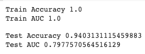
So from the model developed, we can see that the model’s testing parameters are lesser than the training parameters but according to the classification report, the model is possessing an accuracy score of 94%.

Now let us look into how to save this base model in pickle format.

Saving the model in pickle format

In general, the machine learning models are more likely to be saved in a pickle format for easy saving and loading of the saved model parameters. So let us look into the steps involved in saving a machine learning model in pickle format.

import pickle
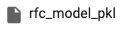
with open('rfc_model_pkl', 'wb') as files:
   pickle.dump(rfc_base, files)

So here the pickle module has been imported to the working environment and a pickle object is created with writable permission operations and the base model developed is dumped in a pickle file format in the pickle object created. So the pickle object created can be checked in the working environment where it will be saved in a pkl format.

Loading the saved model

Now let’s read the saved pickle file in the working environment by following the steps mentioned below.

# load saved model
with open('rfc_model_pkl' , 'rb') as f:
   rfc_pretrained = pickle.load(f)

So here the pickle file created is opened in a readable format (rb) and the load() function of pickle is used to obtain the pretrained model into the working environment.

Obtaining predictions from the saved model

So now the pretrained model can be used to obtain predictions for a random set of parameters, that is passed on to the pretrained model in the same order as the original dataset. The steps to follow for the same are listed below.

rfc_pretrained.predict([[55,0,1,0,2,0,107.93,42,3]])

rfc_pretrained.predict([[81,1,1,1,3,0,100,35.7,3]])

So in this way, we have to pass random features in the respective order of the data frame and obtain predictions for the pretrained model. So in the later stage, this pretrained model is used to evaluate various parameters as shown below.

y_pred_pretrained=rfc_pretrained.predict(X_test)
print('Classification_report of the pretrained model \n',classification_report(Y_test,y_pred_pretrained))

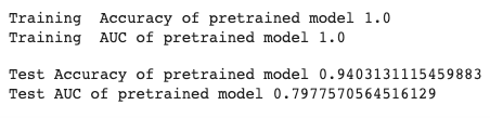
As the classification report of the pretrained model was obtained other parameters of the pretrained model were also evaluated as shown below.

y_train_pred=rfc_pretrained.predict(X_train)
y_train_prob=rfc_pretrained.predict_proba(X_train)[:,1]
y_test_prob=rfc_pretrained.predict_proba(X_test)[:,1]
 
print('Training  Accuracy of pretrained model',accuracy_score(Y_train,y_train_pred))
print('Training  AUC of pretrained model',roc_auc_score(Y_train,y_train_prob))
print()
print('Test Accuracy of pretrained model',accuracy_score(Y_test,y_pred_pretrained))
print('Test AUCo f pretrained model',roc_auc_score(Y_test,y_test_prob))

Summary

So this is how a machine learning model in real-time is built from scratch and saved as standard model formats like pickle and later loaded into working environments to take up predictions for similar kinds of features. Pickle file formats are memory friendly and it provides easy writing and reading operations of the instance created and facilitates obtaining predictions and evaluation of various parameters using the pretrained models.