Geoffrey E Hinton is Canadian cognitive psychologist and computer scientist who is commonly known as the person behind the neural nets or artificial neural networks. He is one of the creators of Deep Learning and has invented various algorithms. He found out a few of the problems that were present in the standard neural networks and tried overcoming those by proposing a completely new neural net algorithm known as “Capsule Networks”. His team also proposed a  new paper that was “Dynamic routing between capsules” that was used to train capsule nets. Convolution neural networks have made remarkable success in the field of computer vision but there are still areas where the network gets in trouble. There are issues in the network that result in poor performance of the network in some of the areas.

This article illustrates the problems with standard neural net and implementation of Capsule Network to overcome the problems. We will first go through the need for such a network and then will implement the CapsNet model in the task of image reconstruction where we will use the MNIST handwritten digit dataset.

What will we discuss in the article?

1. Why do we need Capsule Networks?
2. What is Capsule Networks?
3. How to build Capsule Networks?

1. Why do we need Capsule Networks?

Convolution Neural Network being computationally strong have the ability to automatically detect feature maps from the images. It’s the CNN algorithm that has made it easy for a  machine to do several image-related tasks whether it is about classification or detection. In CNN, the convolution layer holds a very important function that is to detect the features from an image pixel. Deeper ConvNet layers detect the simple features like edges and color. Although the performance of CNN is really good, still they have few of the drawbacks. As quoted by Hinton “The pooling operation used in convolutional neural networks is a big mistake, and the fact that it works so well is a disaster. There is a loss of valuable information when we are using pooling layers. 

Also, CNN requires massive amounts of data to learn. The layers in CNN reduce the spatial resolution and the output of the networks never change even with a small amount of change in the inputs. It cannot directly relate to the relation of parts and requires additional components. This is where Capsule Networks comes into play and overcomes all the drawbacks that are present on CNN.

2. What is Capsule Networks?

Capsule Networks (CapsNet) are the networks that are able to fetch spatial information and more important features so as to overcome the loss of information that is seen in pooling operations. Let us see what is the difference between a capsule and a neuron. Capsule gives us a vector as an output that has a direction. For example, if you are changing the orientation of the image then the vector will also get moved in that same direction whereas the output of a neuron is a scalar quantity that does not tell anything about the direction.

2.1 Architecture of CapsNet on MNIST Data 

2.2 Components of a Capsule Networks

There are 4 main components that are present in the CapsNet that are listed below: 

1. Matrix Multiplication – It is applied to the image that is given as an input to the network to convert into vector values to understand the spatial part.
2. Scalar Weighting of the Input – It computes which higher-level capsule should receive the current capsule output.  
3. Dynamic routing algorithm – It permits these different components to transfer information amongst each other. Higher-level capsules get the input from the lower level. This is a repetitive process. 
4. Squashing Function – It is the last component that condenses the information. The squashing function takes all the information and converts it into a vector that is less than or equal to 1 also maintaining the direction of the vector. 

The architecture consists of 6 layers, first 3 layers are considered to be encoders where the task is to convert the input image into a vector and after that, the last 3 layers are called decoders are used to reconstruct the image using that.

3. How to build a capsule network?

First, we need to define the libraries that are required. Use the below code snippet to import the libraries and import the dataset. The dataset is famous Handwritten digits data that has digits from 0-9.

import numpy as np
import tensorflow as tf
from tensorflow.examples.tutorials.mnist import input_data

mnist = input_data.read_data_sets("/tmp/data/")

After importing the required libraries let add the first input layer that will take the image. We have created a placeholder keeping batch as none with 28×28 pixels and channel as 1. Then we have started the definition of the capsule by defining the first two convents layer after that we have reshaped the output coming to the 2nd ConvNet layer to get the vector of 8D that gives the primary capsule output. The 2nd ConvNet layer contains 32*8 (256) feature maps. Due to which the output shape of the 2nd convent layer is (batch_size, 6 , 6 , 256).  

input_image = tf.placeholder(shape = [None,28,28,1], dtype = float32)
conv1 = tf.layers.conv2D(input_image, 10, kernel_size = 9, stride=1,padding=“none”)
conv1 = tf.layer.conv2D(activation= ‘relu’)
conv2 = tf.layers.conv2D(input_image, 256, kernel_size = 9, stride=2,padding=“none”)
conv2 = tf.layer.conv2D(activation= ‘relu’)
capsule_1= tf.reshape(conv2,[-1,1152,8]) 

After this we have defined the squash function referring to the paper that will squash all these vectors along the defined axis and then we have passed each capsule to this squash function. 

def squash(s, name=None): 
with tf.name_scope(name, default_name="squash"): 
squared_norm = tf.reduce_sum(tf.square(s), axis=-1,     keep_dims=True)
safe_norm = tf.sqrt(squared_norm + 1e-7)
squash_factor = squared_norm / (1. + squared_norm) unit_vector = s / safe_norm return squash_factor * unit_vector
caps1_out = squash(capsule_1)

After this, we define the digit capsule which is a total of 10 in number that outputs 16-dimensional vectors. Let us see how to compute this digit capsule. So, the first step is to compute the predicted output vectors since the second layer is connected to the first layer and we will predict one output for each pair of first and second layer capsules. By making use of the first primary capsule we can predict the output of the first digit capsule. This is done for all the digit capsules using the first primary capsule. Once it is computed we go for the second primary capsule output and compute the digit capsule in a similar fashion. The shape of the first array and second array is  (1152, 10, 16, 8), (1152, 10, 8, 1). The second array should contain 10 identical vectors. To do so we will use the tf.tile() function. Considering batch size to be 32, the network would make predictions for these 32 simultaneously. Therefore the shape of the first array will be (32, 1152,10,16,8) and the shape of the second array would be (32,1152,10,8,1). 

W_init = tf.random_normal(shape=(1, caps1_n_caps, caps2_n_caps, caps2_n_dims, caps1_n_dims), stddev=init_sigma, dtype=tf.float32, name="W_init") W = tf.Variable(W_init, name="W")

batch_size = tf.shape(X)[0] W_tiled = tf.tile(W, [batch_size, 1, 1, 1, 1], name="W_tiled")

We need to create an array of shape (32,1152,10,8,1) that holds the outputs of the first layer capsules, repeated 10 times so we will first enlarge it to get an array of the same shape after which it can iterate or 10 times along the third dimension.

caps1_output_enlarge = tf.expand_dims(caps1_output, -1)
caps1_output_tile = tf.expand_dims(caps1_output_expanded)
caps1_output_tiled = tf.tile(caps1_output_tile, [1, 1, caps2_n_caps, 1, 1])

print(W_tiled)
print(caps1_output_tiled)

Output:-
<tf.Tensor 'W_tiled:0' shape=(?, 1152, 10, 16, 8) dtype=float32>
<tf.Tensor 'caps1_output_tiled:0' shape=(?, 1152, 10, 8, 1) dtype=float32>

As discussed before now will take the product of both the array and check the shape.

caps2_predicted = tf.matmul(W_tiled, caps1_output_tiled)
print(caps2_predicted)

Output:-
<tf.Tensor 'caps2_predicted:0' shape=(?, 1152, 10, 16, 1) dtype=float32>

After this, we will go to the next step that is routing, use the below code snippet to perform 2 round routing and after that, we will define the placeholder for the label. Below image represents the routing algorithm that has been taken from the original paper.

Round 1 Routing: 


raw_weights = tf.zeros([batch_size, caps1_n_caps, caps2_n_caps, 1, 1], dtype=np.float32, name="raw_weights")

routing_weights = tf.nn.softmax(raw_weights, dim=2, name="routing_weights")

weighted_predictions = tf.multiply(routing_weights, caps2_predicted, name="weighted_predictions") weighted_sum = tf.reduce_sum(weighted_predictions, axis=1, keep_dims=True, name="weighted_sum")


Round 2 Routing: 


caps2_output_round_1_tiled = tf.tile( caps2_output_round_1, [1, caps1_n_caps, 1, 1, 1], name="caps2_output_round_1_tiled")

agreement = tf.matmul(caps2_predicted, caps2_output_round_1_tiled, transpose_a=True, name="agreement")

raw_weights_round_2 = tf.add(raw_weights, agreement, name="raw_weights_round_2")

routing_weights_round_2 = tf.nn.softmax(raw_weights_round_2, dim=2, name="routing_weights_round_2")

weighted_predictions_round_2 = tf.multiply(routing_weights_round_2, caps2_predicted, name="weighted_predictions_round_2") 

weighted_sum_round_2 = tf.reduce_sum(weighted_predictions_round_2, axis=1, keep_dims=True, name="weighted_sum_round_2") 

caps2_output_round_2 = squash(weighted_sum_round_2, axis=-2, name="caps2_output_round_2")


 y = tf.placeholder(shape=[None], dtype=tf.int64, name="y")

After computing the routing and placeholder for the label we will define the margin loss that has been mentioned in the original paper to identify two or more unalike digits each image. After that, we have defined the values and did encoding for the labels. In addition to that for output capsule, we have calculated the norm and after that, we have reshaped it to get a matrix of shape (batch size, outputs). After getting the matrix we have computed the loss for each digit and computed the final loss by taking mean. We have assigned the values of m_plus, m_minus and lambda as mentioned in the original paper stated below.

m_plus = 0.9
m_minus = 0.1
lambda_ = 0.5 

T = tf.one_hot(y, depth=caps2_n_caps, name="T")

caps2_output_norm = safe_norm(caps2_output, axis=-2, keep_dims=True, name="caps2_output_norm")

present_error_raw = tf.square(tf.maximum(0., m_plus - caps2_output_norm), name="present_error_raw")

present_error = tf.reshape(present_error_raw, shape=(-1, 10), name="present_error")

absent_error_raw = tf.square(tf.maximum(0., caps2_output_norm - m_minus), name="absent_error_raw")

absent_error = tf.reshape(absent_error_raw, shape=(-1, 10), name="absent_error")

L = tf.add(T * present_error, lambda_ * (1.0 - T) * absent_error, name="L")

margin_loss = tf.reduce_mean(tf.reduce_sum(L, axis=1), name="margin_loss")

After defining the margin loss we now define the decoder part of the network that contains 3 fully connected layers that are responsible for reconstructing the images using the features and information that can be passed in the form of a vector by the encoder. After doing the reconstruction part we will define the decoder and computed reconstruction loss. At last, we have calculated the final loss by merging margin loss and reconstruction loss. The code of the same has been shown below. 

mask_with_labels=tf.placeholder_with_default(False,shape=(),name="mask_with_labels")
reconstruction_targets = tf.cond(mask_with_labels, lambda: y, lambda: y_pred) 

Reconstruction_mask=tf.one_hot(reconstruction_targets,depth=caps2_n_caps,name="reconstruction_mask")

reconstruction_mask_reshaped=tf.reshape(reconstruction_mask,[-1,1,caps2_n_caps, 1, 1], name="reconstruction_mask_reshaped")

caps2_output_masked=tf.multiply(caps2_output,reconstruction_mask_reshaped,name="caps2_output_masked")

decoder_input=tf.reshape(caps2_output_masked,[-1,caps2_n_caps*caps2_n_dims], name="decoder_input")


With tf.name_scope("decoder"): 

hidden1=tf.layers.dense(decoder_input,512,activation=’relu’,name="hidden1")
          hidden2 = tf.layers.dense(hidden1,1024, activation=’relu’, name="hidden2") 
decoder_output=tf.layers.dense(hidden2,28X28,activation=’sigmoid’,name="decoder_output")


X_flat = tf.reshape(X, [-1, n_output], name="X_flat")

squared_difference=tf.square(X_flat-decoder_output,name="squared_difference") reconstruction_loss=tf.reduce_mean(squared_difference,name="reconstruction_loss")

loss = tf.add(margin_loss, 0.001 * reconstruction_loss, name="loss")

Now the final step is to train the capsule network and compute the accuracy and loss. We will be training the network for 10 epochs with a batch size of 32. After 4 epochs the accuracy has reached to 99.4%. 

n_epochs = 10
batch_size = 32
with tf.Session() as sess:
    if restore_checkpoint and tf.train.checkpoint_exists(checkpoint_path):
        saver.restore(sess, checkpoint_path)
    else:
        init.run()
    loss_vals = []
        acc_vals = []
        for iteration in range(1, n_iterations_validation + 1):
            X_batch, y_batch = mnist.validation.next_batch(batch_size)
            loss_val, acc_val = sess.run(
                    [loss, accuracy],
                    feed_dict={X: X_batch.reshape([-1, 28, 28, 1]),
                               y: y_batch})
            loss_vals.append(loss_val)
            acc_vals.append(acc_val)
            print("\rEvaluating the model: {}/{} ({:.1f}%)".format(
                      iteration, n_iterations_validation,
                      iteration * 100 / n_iterations_validation),
                  end=" " * 10)
        loss_val = np.mean(loss_vals)
        acc_val = np.mean(acc_vals)
        print("\rEpoch: {}  Val accuracy: {:.4f}%  Loss: {:.6f}{}".format(
            epoch + 1, acc_val * 100, loss_val)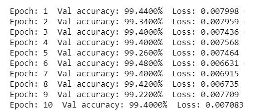

After training, we will evaluate the model by defining a function that computes the validation accuracy and loss. We receive the validation accuracy to be 99.53% with a loss of 0.006.

n_iterations_test = mnist.test.num_examples
loss_tests = []
acc_tests = []
for iteration in range(1, n_iterations_test + 1):
        X_batch, y_batch = mnist.test.next_batch(batch_size)
        loss_test, acc_test = sess.run(
                [loss, accuracy],
                feed_dict={X: X_batch.reshape([-1, 28, 28, 1]),
                           y: y_batch})
        loss_tests.append(loss_test)
        acc_tests.append(acc_test)
        print("\rEvaluating the model: {}/{} ({:.1f}%)".format(
                  iteration, n_iterations_test,
                  iteration * 100 / n_iterations_test),
              end=" " * 10)
    loss_test = np.mean(loss_tests)
    acc_test = np.mean(acc_tests)
    print("\rFinal test accuracy: {:.4f}%  Loss: {:.6f}".format(
        acc_test * 100, loss_test))

We then make predictions using the network. Use the below code to do the same.

sample_images = sample_images.reshape(-1, 28, 28)
reconstructions = decoder_output_value.reshape([-1, 28, 28])

plt.figure(figsize=(n_samples * 2, 3))
for index in range(n_samples):
    plt.subplot(1, n_samples, index + 1)
    plt.imshow(sample_images[index], cmap="binary")
    plt.title("Label:" + str(mnist.test.labels[index]))
    plt.axis("off")
plt.show()

plt.figure(figsize=(n_samples * 2, 3))
for index in range(n_samples):
    plt.subplot(1, n_samples, index + 1)
    plt.title("Predicted:" + str(y_pred_value[index]))
    plt.imshow(reconstructions[index], cmap="binary")
    plt.axis("off")
plt.show()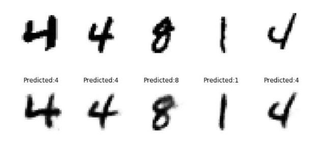

Conclusion 

As capsule networks have received the state of the art performance on the image reconstruction of MNIST dataset but still they lagged behind when we use them for more complex datasets. You can also read here the similar context article that is “Why do capsule networks work better than CNN”. There are lots of features present in the data like ImageNet and Coco and this is the reason why CapsNets fail miserably here. Capsule Networks are still in the Research and Development stage and people cannot rely on them to use for complex data or complex tasks while dealing with images. 

 References:- 

1. Aryan Misra, “Capsule Network, The Deep Learning Network” 
2. Aurélien Geron, “How to Implement CapsNets using tensorflow”