Bayesian statistics is one of the most popular concepts in statistics that are widely used in machine learning as well. Many of the predictive modelling techniques in machine learning use probabilistic concepts. When we need to find the probability of events that are conditionally dependent on each other, the Bayesian approach is followed there. In this post, first, we will interpret different types of events and their probabilities in the context of the Bayes theorem and then we will do hands-on experiments in python to find the probabilities of events using the Bayesian approach. The major points to be covered in the article are listed below.
Table of Contents
- Bayes Theorem
- Prior Probability
- Likelihood Function
- Posterior Probability
- Bayesian Statistics in Python
Bayes Theorem
The Bayes theorem can be understood as the description of the probability of any event which is obtained by prior knowledge about the event. We can say that Bayes’ theorem can be used to describe the conditional probability of any event where we have data about the event and also we have prior information about the event with the prior knowledge about the conditions related to the event. For example, when we talk about statistical models such as logistic regression we can consider them as the probability distribution for the given data, and for this model, we can use the Bayes theorem to estimate the parameters of the model.
Since the probabilities in the Bayesian statistics can be treated as a degree of belief, we can directly assign the probability distribution that can generate the belief to the parameter (or set of parameters) by quantifying them using the Bayes theorem. Mathematically the Bayes theorem can be expressed as

Where A and B are two events. To explain it more, let’s take an example. We have two bags given A and B each consisting of a few coloured balls. If a red ball is drawn, to find the probability that it is drawn from bag A, we can use the Bayes theorem. It finds out the probability of a prior event given that the posterior event has already occurred.
Prior probability
In the formula of the Bayes theorem, P(A) is the prior probability of A. We can define the prior probability or prior as the probability distribution of any uncertain quantity which is an expression of one’s belief about uncertain quantity without or before taking any evidence into account. For example, huge numbers of balls need to be distributed in buckets and we can consider a probability distribution as prior if the distribution is representing the proportion of balls that will take place in a particular bucket. The example of an unknown quantity can be a parameter of any statistical model. By the formula P(A) expresses one’s belief of occurrence of A before any evidence is taken into account.
Likelihood Function
In the formula of Bayes theorem, P(B|A) is the likelihood function which can be simply called the likelihood which can be defined as the parameter functions of any statistical model which helps in describing the joint probability of the observed data. It can be more simplified as the probability of B when it is known that A is true. Numerically it is the support value where the support to proposition A is given by evidence B.
Posterior Probability
In the formula of the Bayes theorem, P(B|A) is a posterior probability that can be defined as the conditional probability of any random event or uncertain proposition when there is knowledge about the relevant evidence that is present and taken into account. According to the Bayes theorem probability formula, this value represents the probability of A when evidence B has been taken into account.
From the above intuitions and definitions, we can say that the Bayes theorem can be written as the posterior probability will be equal to the product of likelihood probability, prior probability, and the inverse of the probability of evidence(B) being true.
Next in the article, we will take an example so that we can understand how these basic Bayesian statistics works and how we can perform them in python.
Bayesian Statistics in Python
Let’s take an example where we will examine all these terms in python.
For example, suppose we have 2 buckets A and B. In bucket A we have 30 blue balls and 10 yellow balls, while in bucket B we have 20 blue and 20 yellow balls. We are required to choose one ball. What is the chance that we choose bucket A?
We can say that there is an equal chance for choosing either of the buckets but now from the chosen bucket we picked a blue ball, so the question is what is the chance we pick it from bucket A?
Let’s solve it with python.
#Importing libraries
import numpy as np
import pandas as pd
import matplotlib.pyplot as plt
import seaborn as sns
According to the question, the hypotheses and prior are:
hypos = 'bucket a', 'bucket b'
probs= 1/2,1/2
We can use the pandas series for computation as:
prior = pd.Series(probs, hypos)
print(prior)
Output:

Here the series represents the probability mass function which can be defined as the probability distribution of a random variable that is discrete; more simply, we can consider it as a tool for defining a discrete probability distribution.
According to the question, we know that the chances of choosing a blue ball from bucket A is ¾ and from bucket B the chances of choosing any ball or blue ball are ½. This chance or probabilities are our likelihood.
So from the above statement, we can say that,
likelihood = 3/4, 1/2Using the likelihood and prior we can calculate the unnormalized posterior as:
unnorm = prior * likelihood
print(unnorm)
Output:

To make the unnormalized posterior normalized posterior we have to divide the unnormalized posterior with the sum of the unnormalized posterior.
prob_data = unnorm.sum()
prob_data
Output:

posterior = unnorm / prob_data
posterior

Here from the results, we can say the posterior probability of choosing bucket A with a blue ball is 0.6. Which is an implementation of the Bayes theorem which we had read above.
Now suppose a similar situation as given in the above problem, putting back the previous lifted block and choosing a ball from the similar bucket and it is a yellow ball. Now, what is the probability that both times we chose bucket A to pick the ball?
Here we can say that the posterior we computed from the first problem can be prior to this problem which means
prior = posterior
print(prior)
The likelihood for these problems are:
likelihood = 3/4, 1/2Unnormalized posterior are:
unnorm = prior * likelihood
print(unnorm)
Output

Sum of unnormalized posteriors:
prob_data = unnorm.sum()
prob_data
Output:

Posterior probabilities:
posterior = unnorm / prob_data
print(posterior)
Output:

Here we can see that the posterior probability for bucket A in the second attempt is 0.428571.
It is necessary that the computed posterior probabilities add up to 1. The reason behind this is very simple: the hypotheses are “complementary”; which means that only one of the situations can be true either first or second, both cannot be true. Summing the unnormalized posterior makes the posterior to add up to 1 only
Let’s increase the complexity of the problem this time we have 101 buckets and the distribution of the balls are like below given points :
- Bucket 0 has the o blue balls
- Bucket 1 has 1% blue balls
- Bucket 2 has 2% blue balls
And so on up to
- Bucket 99 has 99% blue balls
- Bucket 100 has 100% blue balls.
In the previous example, we had only two types of buckets. Now in this problem, we have 100% yellow balls in bucket 0 and 99% yellow balls in bucket 1 and so on.
Now suppose we randomly choose a bucket and pick a ball and it turns out to be blue. What is the probability that the ball came from Bucket ????, for each value of ?????
To solve this problem we can make a series of numbers 0 to 100 where the numbers are equally spaced with each other.
xs = np.linspace(0, 1, num=101)
prob = 1/101
prior = pd.Series(prob, xs)
prior.head()
Output:
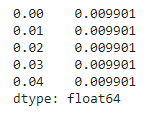
As the problem is given, we can check our priors with the distribution of blue balls by visualization.
prior.plot()
plt.xlabel('Fraction of blue balls')
plt.ylabel('Probability')
plt.title('Prior');
Output:

We can say that the likelihood for the blue balls will be equal to the distributed numbers in the xs.
likelihood_blue = xs
print(likelihood_blue)
Output:

The likelihood for the yellow balls:
likelihood_yellow = 1-xs
print(likelihood_yellow)
Output:

The unnormalized posterior for this situation will be:
unnorm = prior * likelihood_vanilla
print(unnorm)
Output:
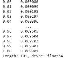
And the posterior for picking a blue ball will be:
posterior = unnorm / unnorm.sum()
The posterior for blue ball cookie came from bucket ????, for each value of ???? look like:
posterior.plot()
plt.xlabel('Fraction of blue balls')
plt.ylabel('Probability')
plt.title('Posterior, one blue ball');
Output:
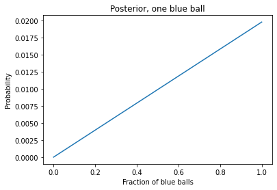
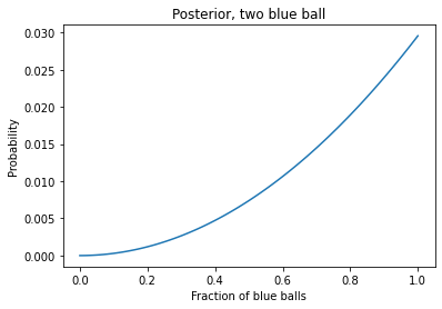
Let’s do the same thing again, put the ball back and pick the ball from the same bucket and get a blue ball now. What will be the posterior?
Here again, we can say the posterior from the above problem will the prior in the below procedure:
prior = posterior
unnorm = prior * likelihood_vanilla
posterior = unnorm / unnorm.sum()
Plotting the posterior.
posterior.plot()
plt.xlabel('Fraction of blue balls')
plt.ylabel('Probability')
plt.title('Posterior, two blue ball');
Output:
Now suppose we put the ball again in the bucket and again pick a ball and get a yellow ball. Now, what are the posterior probabilities?
prior = posterior
unnorm = prior * likelihood_yellow
posterior = unnorm / unnorm.sum()
Plotting the posterior:
posterior.plot()
plt.xlabel('Fraction of yellow ball')
plt.ylabel('Probability')
plt.title('Posterior, two blue ball, one yellow ball');
Output:
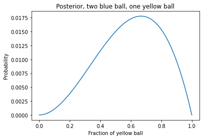
Here we can see the posteriors for the situation where we get a yellow ball.
Final Words
Here in the article, we have seen the Bayes theorem which is basically a part of Bayesian statistics along with we have an introduction with the terminologies like prior, likelihood, posterior which are not only useful in making the Bayes theorem but also have a huge number of application in the complex Bayesian statistics. There are various applications of Bayesian statistics like survival analysis, statistical modelling, parameter estimation e, etc. I encourage the readers to go more in-depth to utilize it with real-life applications because the results we get from this type of statistical analysis are mostly simple and accurate.
References


