The data which changes according to time has trends and seasonality which make the data non-stationary. To check the stationarity of data there are certain statistical methods to compute the hypothetical question answering. In this article, we will be discussing the commonly used statistical methods to compute stationarity of the time series data and conversion of non-stationary to stationary series. Following are the topics to be covered.

Table of contents

1. The necessity of time series to be stationary
2. Statical methods to check stationarity
3. Making time series stationary using python
4. Converting non-stationary to stationary

Let’s start with the necessity of stationary time series.

The necessity of time series to be stationary

Most time series models presume that each point is independent of the others for forecasting or predicting the future which means the mean, variance, and covariance do not change over time. When the dataset of previous cases is steady, this is the best indicator. 

The statistical features of a system must not vary over time for data to be stationary. This does not imply that the values for each data point must be the same, but that the general behaviour of the data must be consistent. Time graphs that do not indicate patterns or seasonality might be termed stagnant on a strictly visual basis. 

A constant mean and a constant variance are two more numerical elements that support stationarity. There are two important terms related to time series data.

• When there is a long-term growth or decrease in the data, this is referred to as a trend.
• A recurring pattern with a defined and predictable regularity dependent on the time of year, week, or day is referred to as seasonality.

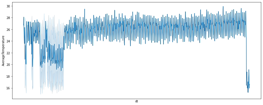
The representation below shows a clear example of non-stationary data. The figure exhibits a significant upward trend and seasonality. Although this provides a wealth of information about the data’s qualities, it is not stationary and hence cannot be anticipated using typical time series models. The spread of the data indicates that there is a significant variation in the data. To flatten the growing variance, we need to transform the data.

Are you looking for a complete repository of Python libraries used in data science, check out here.

Statical methods to check stationarity

There are two common statistical methods used to check the stationarity of time series data.

Augmented Dickey-Fuller Test:

The Augmented Dickey-Fuller Test (ADF) is a stationarity unit root test. The ADF test is a modified version of the Dickey Fuller exam. In the time series analysis, unit-roots might produce unexpected findings.

With serial correlation, the Augmented Dickey-Fuller test may be utilized. The ADF test is more powerful and can handle more complicated models than the Dickey-Fuller test. However, like with other unit root tests, it should be used with caution because it has a somewhat high Type I error rate.

The following are the test hypotheses:

• Null hypothesis (H0): The time series data is non-stationary.
• Alternate hypothesis (H1): The time series is stationary (or trend-stationary).

The ADF test extends the Dickey-Fuller test equation to include in the model a high order regressive process. It adds extra differencing terms, but the rest of the equation stays unchanged. This increases the thoroughness of the test.

The null hypothesis, on the other hand, remains the same as in the Dickey-Fuller test.

To reject the null hypothesis, the p-value produced should be less than the significance level (say, 0.05). As a result, we may conclude that the series is stationary.

Kwiatkowski Phillips Schmidt Shin (KPSS) test:

The Kwiatkowski Phillips Schmidt Shin (KPSS) test determines if a time series is stationary around a mean or linear trend, or non-stationary as a result of a unit root. A stationary time series has statistical features such as mean and variance that remain constant across time.

The following are the test hypotheses:

• Null hypothesis (H0): The data is stationary.
• Alternate hypothesis (H1): The data is not stationary.

The linear regression underpins the KPSS test. With the regression equation, it divides a series into three parts: a deterministic trend, a random walk, and a stationary error. If the data is stationary, the intercept will have a fixed element or the series will be stationary around a fixed level. 

The test uses OLS to compute the equation, which varies significantly depending on whether you want to test for level or trend stationarity. To assess level stationarity, a reduced version lacking the temporal trend component is used.

Making time series stationary using python

Implementing the above mentioned techniques in python by using the statsmodel library.

Import necessary libraries and data for processing:

import pandas as pd
import numpy as np
import matplotlib.pyplot as plt
import seaborn as sns
import warnings
warnings.filterwarnings("ignore")
 
from statsmodels.tsa.stattools import adfuller
from statsmodels.tsa.stattools import kpss
df_new=pd.read_csv("GlobalLandTemperatures_GlobalLandTemperaturesByMajorCity.csv")
df_utils_new=df_new[['dt','AverageTemperature']]
df_utils_new[:8]

fig=plt.figure(figsize=(15,6))
sns.lineplot(data=df_utils,x='dt',y='AverageTemperature')
plt.tick_params(
    axis='x',        
    which='both',   
    bottom=False,      
    top=False,        
    labelbottom=False) 
plt.show()

Augmented Dickey-Fuller Test:

result=adfuller (df_use['AverageTemperature'])
print('Test Statistic: %f' %result[0])
print('p-value: %f' %result[1])
print('Critical values:')
for key, value in result[4].items ():
     print('\t%s: %.3f' %(key, value))

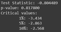
As the test statistic is greater (less negative) then the critical value becomes the reason to not reject the null hypothesis. This indicates that the data is non-stationary.

Kwiatkowski Phillips Schmidt Shin (KPSS) test:

result_kpss_ct=kpss(df_use['AverageTemperature'],regression="ct")
print('Test Statistic: %f' %result_kpss_ct[0])
print('p-value: %f' %result_kpss_ct[1])
print('Critical values:')
for key, value in result_kpss_ct[3].items():
     print('\t%s: %.3f' %(key, value))

Here checking the KPSS statistics on the trend of the data, so the regression is “ct”.

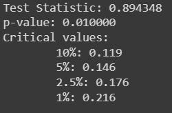
As the test statistics value is greater than the critical value, the null hypothesis is rejected. This indicates that the data is non-stationary.

Let’s see if the data is non-stationary and the ways to transform the data to stationary.

Converting non-stationary to stationary

To detrend the time series data there are certain transformation techniques used and they are listed as follows.

• Log transforming of the data
• Taking the square root of the data
• Taking the cube root
• Proportional change

The steps for transformation are simple, for this article uses square root transformation.

1. Use NumPy’s square root function to transform the required column
2. Then shift the transformation by one using the “shift’ function.
3. Take the difference between both the original transformation and shift.
4. Steps 2 and 3 can be done by just using the pandas “diff” function.

Use the below code to obtain the above-mentioned steps.

Transforming the data

df_log=np.sqrt(df_use['AverageTemperature'])
df_diff=df_log.diff().dropna()

Checking the stationarity

result=adfuller (df_diff)
print('Test Statistic: %f' %result[0])
print('p-value: %f' %result[1])
print('Critical values:')
for key, value in result[4].items ():
     print('\t%s: %.3f' %(key, value))

As the ADF test statics is lesser (more negative) then the critical value becomes the reason to reject the null hypothesis. This indicates that the data is stationary.

result_kpss_ct_log=kpss(df_diff,regression="ct")
print('Test Statistic: %f' % np.round(result_kpss_ct_log[0],2))
print('p-value: %f' %result_kpss_ct_log[1])
print('Critical values:')
for key, value in result_kpss_ct_log[3].items():
     print('\t%s: %.3f' %(key, value))

As the KPSS test statistics value is less than the critical value, the null hypothesis is not rejected. This indicates that the data is stationary.

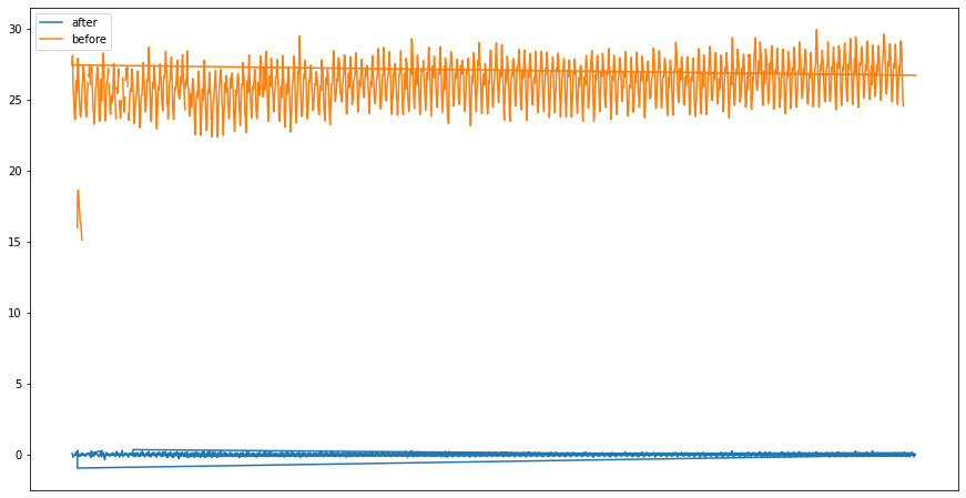
Comparing the after and before versions of time series

plt.figure(figsize=(15,8))
plt.plot(df_diff,label="after")
plt.plot(df_compare,label="before")
plt.tick_params(
    axis='x',        
    which='both',   
    bottom=False,      
    top=False,        
    labelbottom=False)
plt.legend()
plt.show() 

Conclusion

A time series whose statistical properties such as mean, variance, autocorrelation, etc. are all constant over time is referred to as stationary. Because a stationary series is generally simple to anticipate, it can be “untransformed.” Any prior mathematical modifications used to produce predictions for the original series could be reversed. With this article, we have understood different techniques to detect the stationarity of time series data and to transform non-stationary data into stationary time series.

References

• Link to the above code
• Read about ADF test
• Read about KPSS test
• Documentation for statsmodel