In time series analysis and modelling, detrending plays a crucial role because it makes us acquainted with the cyclic and other patterns of the time series. The process of detrending involves the removal of the trend effect from time series to identify the differences in values from the trend. Using various filters like Band-Pass Filter, Baxter-King Filter (BK Filter), and  Hodrick–Prescott filter we can perform the detrending of the time series. In this article, we will discuss one of these filters for time series detrending, the Hodrick–Prescott (HP) filter, in detail with its practical implementation. The major points to be discussed in this article are listed below.

Table of contents 

1. About Hodrick–Prescott filter
2. How does the Hodrick–Prescott filter work?
3. Implementing Hodrick–Prescott filter in python
4. Advantages of Hodrick–Prescott filter
5. Limitations of Hodrick–Prescott filter 

Let’s start the discussion by understanding the Hodrick–Prescott filter.

About Hodrick–Prescott filter

The Hodrick–Prescott filter or Hodrick–Prescott decomposition is a mathematical tool that is used in time series analysis and modelling. This filter is mainly useful in removing the cyclic component from time-series data. Applying the Hodrick–Prescott filter in time series allows us to obtain a smooth time series from time series that has time series components like trend cycle and noise in large quantities. This filter is named before the names of economists Robert J. Hodrick and Edward C. Prescott.   

How does the Hodrick–Prescott filter work?

Mathematically, the basic idea behind this filter is related to concepts in the decomposition of time series. Let’s understand this mathematically by taking an example of time series y_t.

Where,

In y_t

t = 1, 2, 3,…..,T

𝛕_t = trend component 

c_t = cyclic component 

𝜺_t = noise component .

The short-term fluctuations of the time series trend component can be adjusted by using a multiplier . the trend component of time series will solve:

The first term of the equation penalizes the cyclic component, and the second term of the equation penalizes the growth rate of the trend component which can also be compared with the . so if increases that means penalty increases. According to the Hodrick-Prescott filter the value of for a data of 3 months should be 1600. In practice the value of for one year should be 100 and 14,400 if the data is monthly. 

The Hodrick-Prescott filter can be given by,

From the above equation, we can say that the HP filter is not casual because the lag operator L can be seen from F.O.C. for the minimization problems.

Implementing Hodrick–Prescott filter in python

In the above sections, we have gone through the introduction to the HP filter. In this section, we will look at how we can implement it in python. For this we can use the statsmodel library. Using this library we can utilize many functions and modules for the estimation of many different statistical models. This library also provides a module for the HP filter in the statsmodels.tsa.filters package.  

Using this module from statsmodel we can remove the smooth trend from our data. Where if 

T = trend and x = series then the module solves it as:

min (sum((x[t] – T[t])**2 + lamb*((T[t+1] – T[t]) – (T[t] – T[t-1]))**2))

The implementation of this filter can be compared to the ridge regression rule that uses scipy.sparse. By this, we can also write the solution from the module as 

T = inv(I + lamb*K’K)x

Where,

l = nobs

x = nobs identity matrix

k = (nobs-2) x nobs matrix

We can find more details about the module here.

Let’s see how we can perform this. In the implementation, we will also use the practice data from the statsmodel library.

Importing libraries 

import statsmodels.api as sm
import pandas as pd
import matplotlib.pyplot as plt

Loading data 

#importing data
data = sm.datasets.macrodata.load_pandas().data
#making index
data.set_index(pd.period_range('1959Q1', '2009Q3', freq='Q'), inplace = True)

Checking data 

data.columns

Output:

These are the columns we have in the dataset. From these columns, we will be working on the realgdp column. More information on the data can be found in the below output:

print(sm.datasets.macrodata.NOTE)

Output:

Let’s see how the realgdp variable of the data is going with time.

fig, ax = plt.subplots()
data['realgdp']["2000-03-31":].plot(ax=ax,fontsize=12)

Output:

In the image, we can clearly see that the growth of the realgdp time series is not smooth. By this plot, we can say that there are trends and cyclic components are presented in our time series data. 

Now to deal with it, we can use the HP filter for segregating the time series into its components. 

from statsmodels.tsa.filters.hp_filter import hpfilter
gdp_cycle,gdp_trend = hpfilter(data['realgdp'], lamb=1600)
gdp_segr = data[['realgdp']]
gdp_segr['cycle']= gdp_cycle
gdp_segr['trend'] = gdp_trend
gdp_segr

Output:

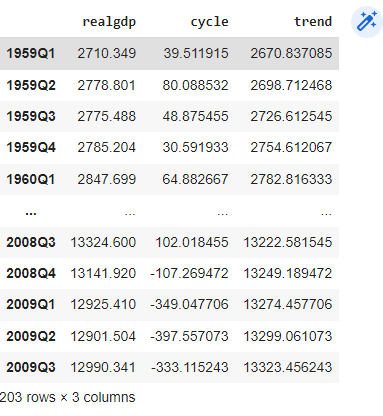
Here in the output, we can see that we have separated the cycle and trend component from the time series. Let’s draw them one by one. 

gdp_trend.plot()

Output:

Here we can see that as we have discussed above we have a smooth trend which we have extracted from the raw time series.

Let’s see how the cyclic component is going with time.

gdp_cycle.plot()

Output:

Here we can see the cyclic component of the time series. Let’s draw all of them together so that we can have a clear vision of the time series.

fig, ax = plt.subplots()

gdp_seg[['realgdp', 'trent', 'cycle']]["2000-03-31":].plot(ax=ax,fontsize=12)

Output:

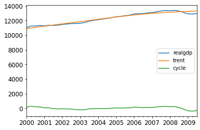
In the above output, we can see a comparative visualization of our time series and its component. Since we use an HP filter to extract the smooth trend from the time series that can be used to make forecasts by ignoring the cyclic component. So it will be much better for us to visualize a comparative graph of time series and extracted trends that can be done using the following codes.

fig, ax = plt.subplots()
gdp_seg[['realgdp', 'trent']]["2000-03-31":].plot(ax=ax,fontsize=12)

Output:

In the above output, we can easily compare between the different lines, and also we can see that now the trend of the time series is actually smoother than the older time series. This trend extraction or detrending allows us to forecast more accurate value. 

Advantages of Hodrick–Prescott filter 

Some of the advantages of the HP filter are as follows:

• Since it is a powerful tool for data smoothing we can use it in macroeconomics.
• It has the capability of removing the fluctuation in short-term time series. So we can easily apply it for short-term time series analysis. 
• It tends to have good results in situations where noise is distributed normally.

Limitations of Hodrick–Prescott filter 

Some of the limitations of the HP filter are as follows:

• To make the HP filter work properly we are required to have data in one trend because the presence of a split growth rate makes the filter generate synthetic shifts in the trend.
• We can perform only static time series analysis using this filter because in a dynamic setting this filter changes the past state of the time series which causes misleading predictions.
• This filter is not backward-looking because its lag operator can be seen from F.O.C. for minimization problems, and that makes it not casual.
• The one-sided version of the HP filter provides smoothing to the time series but it is not capable of extracting values that are not necessary for forecasting.

Final words

In this article, we have discussed the Hodrick-Prescott filter or HP-filter which is mainly used for detrending the time series. We have discussed how we can implement it practically using python. Along with these, we have also discussed its advantages and limitations.      

References

• Statsmodel documentation
• Link for the codes