One of the most useful popular libraries of the python programming language used for machine learning is scikit-learn. The reason behind this popularity is that it consists of simple and efficient tools for classification, regression, clustering, dimensionality reduction, model selection, etc. On 8th September 2021, the new version of scikit-learn, scikit-learn 1.0, was released with new exciting features. In this article, we have covered all the useful and important updates of the new version of scikit-learn. We will go through each of the additions and updates one by one and will try to understand how these updates can make the machine learning process more efficient. The major updates that we will discuss here are listed below.
Table of Contents
- New Features in SKLearn Calibration
- New Features in Feature Selection
- New Features and Models in Linear models
- New Metrics
- New Model Selection Method
- Updates in Data Preprocessing
Now let us go through the new features added to the latest version.
New Features in SKLearn Calibration
The following new calibration features are added in SciKit-Learn 1.0:-
Calibration Curves
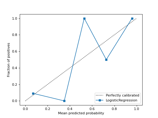
Probabilities Calibration is a rescaling process that is applied after the predictions have been made by a predictive model. The SciKit-Learn 1.0 has a new feature to draw the Calibration curve or reliability diagram. We can draw probability calibration between true labels of the data and predicted labels of the binary classification model or we can draw it using an estimator and the data.
We can plot this curve using the CalibrationDisplay.from_prediction module wherein the module we just need to give real value and predicted value instances as the parameter or CalibrationDisplay.from_estimator module where the parameters accepted will be classifier instance and instances of the dependent and independent variables of the data.
The below image represents the probability calibration between the estimator and the data. Where the estimator is a logistic regression model and data is randomly chosen data points from the make_classification module of sklearn.
New Features in Feature Selection
The following new features on feature selection are added to the scikit learn’s new version:-
Pearson’s R correlation coefficients
The Pearson correlation coefficient or Pearson’s r is a measurement of the linear relationship between the variables in any dataset. It can be measured by dividing covariance by the product of their standard deviations. Using the new feature (feature_selection.r_regression) we can calculate the Pearson’s r between each feature variable and the target variable of the data. Before this update, it used to be in the procedure of feature selection. Now using this module we can make it a free procedure for feature selection.
In the procedure of computing Pearson’s r module uses the following formula:
((X[:, i] - mean(X[:, i])) * (y - mean_y)) / (std(X[:, i]) * std(y))Where X is the features of the dataset and y is the target variable.
Before this feature, we were using the SelectKBest module for selecting the best features using univariate statistical tests where we have options for chi-square test, F-value, and ANOVA F-value test for classification models and F-statistics. P-value and Mutual information test for the regression model.
New Features And Models in Linear Models
The following new features are added related to linear models in SciKit-Learn 1.0:-
- Linear Quantile Regression with L1 Penalty
Quantile regression estimates the other quantiles of the target variable. Quantile regression is a type of regression analysis in which the method of least squares estimates the quantiles of the target variable across values of the feature variables. Using this analysis with L1 regularization which helps in handling the sparsity of the data makes the model predict conditional quantiles more accurately because lowering the high dimensional features makes the data compact and produces quantiles with a higher number of data points. This update provides the model for Quantile Regression combined with L1 regularization.
We can make an instance of this model using sklearn.linear_model.QuantileRegressor command line, where the main parameters are quantile which can be any value between 0 to 1 and according to that the percentage of data can be put in the Quantile i.e. median for example if provided 0.6, the model will predict 60% quantile. Alpha is a parameter for multiplying the L1 penalty term for regularization of the sparsity by default it is set to one.
from sklearn.linear_model import QuantileRegressor
qua_reg = QuantileRegressor(quantile=0.6).fit(X, y)
The above command can be an example of setting an instance for sklearn 1.0 provided Quantile Regression model.
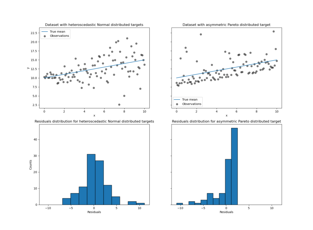
In the above image, we have two datasets with randomly generated data points for regression added with heteroscedastic normal noise(first data set) and asymmetric Pareto noise(second data set.

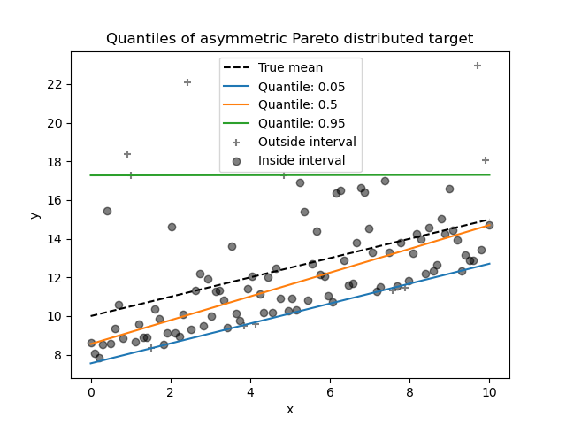
The above image represents an example of how this model can predict non-trivial conditional quantiles on datasets added with heteroscedastic normal noise and asymmetric Pareto noise.
Pinball Loss Function
This new update has added a metric to calculate the pinball loss function. This function is used to assess Quantile prediction accuracy. To calculate the pinball loss function we use the following function.

Where Ƭ is the target quantile and ???? the real value and z is the quantile prediction. Lower pinball loss indicates high accuracy of the quantile prediction. The pinball loss function is always positive and away from the target.
We can implement a pinball loss function using SciKit-Learn 1.0’s provided mean_pinball_loss module in the sklearn.metrics package.
from sklearn.metrics import mean_pinball_loss
mean_pinball_loss(y_true, y_pred)
The above-given lines can be used for calculating the pinball loss between the given target value and the estimated target value.
- SGD Implementation of the Linear One-Class SVM
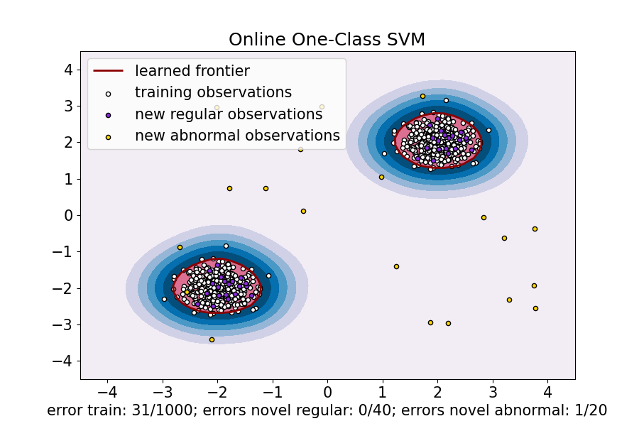
We use One-Class SVM for unsupervised outlier detection which basically checks the support of high dimensional distribution while modelling and with a linear kernel distribution of the data can be done with one line. When a one-class SVM comes with a linear kernel and the dimensionality of the data is high it requires higher effort in calculating the distribution and distribution can be more inaccurate.
Stochastic gradient descent(SGD) replaces the actual gradient of the whole data with an estimated gradient of the sub-data of the data. Especially in high-dimensional optimization problems, this reduces the computational burden, achieving faster iterations merging with One-Class SVM using a linear kernel makes the process healthier and faster.
The new update provides the model for SGD implementation on the linear One-Class SVM. We can use this model from the linear_model package of sklearn where the model name is defined as SGDOneClassSVM.
Following line can be used for making an instance of SGDOneClassSVM:
from sklearn import linear_model
clf = linear_model.SGDOneClassSVM(random_state=42)
The below image represents the outlier detection in the randomly collected dataset where some novel and abnormal observations are randomly presented.
- Sample Weight in Regularization
When working with sequential analysis like time series and NLP data. sometimes we require to decay the data if it is dense before regularization of the data and for that, we did not have any sample weight kind of parameters to define this makes the regularization proceed on the whole data in the new update we have sample_weight parameter in ElasticNet and Lasso regularizer.
- lbfgs Solver for Ridge Regularization
In the update, we have got new solver lbfgs in Ridge and a positive argument which is only supported by the lbfgs only. When positive = True, the solver forces the coefficient to be positive.
New Metrics
The following new metrics are added to the scikit learn’s new version:-
- D2 regression score for Tweedie deviances
McFadden’s R2 also known as the likelihood-ratio index helps in comparing the likelihood for the intercept-only model to the likelihood estimation for the model by the predictors. It is also known as the D² score, or the coefficient of determination is a generalization of the r-square which can be calculated by the following formula.

like r-square it can be negative in case the model is being arbitrarily worse. The squared error of the r-square is replaced by the Tweedie deviance.
In SciKit-Learn 1.0 we have a facility to use the D^2 regression score function, percentage of Tweedie deviance explained. It can be used by the scikit-learn’s provided d2_tweedie_score module in the sklearn.metrics package.
from sklearn.metrics import d2_tweedie_score
d2_tweedie_score(y_true, y_pred)
The following command line can be used for calculating this metric where y_true is given target data and y_pred is estimated values.
- RMSLE (Root Mean Squared Log Error)
In many contests there is a need of finding RMSLE (root mean squared log error) between the true and predicted value so scikit learn has provided mean_sqared_log_error by giving the argument squared = False using which it will calculate the square root of mean_square_log_error so that it can be root_mean_square_log_error.
from sklearn.metrics import mean_squared_log_error
mean_squared_log_error(y_true, y_pred, squared=False)
Using the above command we can calculate the root_mean_square_log_error between target and predicted values.
New Model Selection Method
The following new model selection methods are added to the scikit learn’s new version:-
Stratified Group K-Fold Cross-Validation
The new update facility for model selection using stratified k-fold cross-validation with no overlapping group technique has been introduced in the library. Which is a variant of stratified cold which attempts to return folds with overlapping groups. It preserves the same percentage of samples from each class to make the folds.
Where the groupKFold makes the folds so that the number of different classes is approximately the same on each fold. StratifiedGroupKFold tries to preserve the percentage of samples from each class as much as possible given the constraint of non-overlapping groups between splits.
But when the number of groups has a large number of samples the StratifiedGroupKFold behaves like the GroupKFold because the stratification of samples is not possible.

The above image represents the randomly picked data with three classes and t0 groups. Where the data is in a 1:3:6 ratio in different classes.
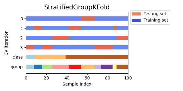
The above image represents the folds of training and testing data on the above-given dataset where the split count is 4. made by StratifiedGroupKFold.
We can implement it in our dataset using the SciKit-Learn 1.0 provided StratifiedGroupKFold module in the model_selection package.
from sklearn.model_selection import StratifiedGroupKFold
cv = StratifiedGroupKFold(n_splits=3)
The above commands can be used for making 3 folds using StratifiedGroupKFold.
Updates on Data Preprocessing
The following updates on data preprocessing are added to the scikit learn’s new version:-
- B-Splines
In the new update, we have a new tool for the generation of B-splines. A spline function of order n is a piecewise polynomial function of degree n-1 in a variable x where B-spline is a spline function that has minimal support with respect to a given degree, smoothness, and domain partition. The meeting point of the pieces is called a knot.
Using SplineTransformer we can generate the B-spline of the features and the parameters under it are:
n_knots – number of knots.
degree – polynomial degree of the spline.
knots – knot positioning strategy.
Using the extrapolation argument we can generate periodic splines and it also supports sample weights for a knot positioning strategy.
from sklearn.preprocessing import SplineTransformer
spline = SplineTransformer(degree=2, n_knots=3)
Using the above command we can generate an instance to generate the b-spline where the number of knots is 3 and the degree of the spline is 2.
- Handle unknown category- If there is any unknown category in the dataset we can consider it as the unknown category using the
OneHotEncoderusing thehandle_unknown = ‘ignore’argument
- Using a new update in the PolynomialFeatures module we can pass a tuple to a degree.
Final Words
Here in the article, we have seen how some of the very new features have been updated in the newer version of scikit learn. Some of the features are like Quantile regression with L1 regularization which is a whole process that needs to be performed step by step but SciKit-Learn 1.0 made it a one-step process. These features are absolutely free and ready to use. I encourage readers to get hands-on with those new things also. They are such very different things. Prior knowledge of these updates can make a person stand out from the crowd.
References:


