When we make a model for forecasting purposes in time series analysis, we require a stationary time series for better prediction. So the first step to work on modeling is to make a time series stationary. Testing for stationarity is a frequently used activity in autoregressive modeling. We can perform various tests like the KPSS, Phillips–Perron, and Augmented Dickey-Fuller. This article is more focused on the Dickey-Fuller test. The article will see the mathematics behind the test and how we can implement it in a time series.

ADF (Augmented Dickey-Fuller) test is a statistical significance test which means the test will give results in hypothesis tests with null and alternative hypotheses. As a result, we will have a p-value from which we will need to make inferences about the time series, whether it is stationary or not.

Before going into the ADF test, we must know about the unit root test because the ADF test belongs to the unit root test.

Unit Root Test

A unit root test tests whether a time series is not stationary and consists of a unit root in time series analysis. The presence of a unit root in time series defines the null hypothesis, and the alternative hypothesis defines time series as stationary.

Mathematically the unit root test can be represented as  

Where,

• Dt is the deterministic component.
• z_t is the stochastic component.
• ɛ_t is the stationary error process.

The unit root test’s basic concept is to determine whether the z_t (stochastic component ) consists of a unit root or not.

There are various tests which include unit root tests.

• Augmented Dickey-Fuller test.
• Phillips-perron test.
• KPSS test.
• ADF-GLS test
• Breusch-godfrey test.
• Ljung-Box test.
• Durbin-watson test.

 Let’s move into our motive, which is the Dickey-Fuller test.

Explanation of the Dickey-Fuller test.

A simple AR model can be represented as:

where

• y_t is variable of interest at the time t
• ρ is a coefficient that defines the unit root
• u_t  is noise or can be considered as an error term.

If ρ = 1, the unit root is present in a time series, and the time series is non-stationary.

If a regression model can be represented as 

Where 

• Δ is a difference operator.
• ẟ = ρ-1

So here, if ρ = 1, which means we will get the differencing as the error term and if the coefficient has some values smaller than one or bigger than one, we will see the changes according to the past observation.

There can be three versions of the test.

• test for a unit root

• test for a unit root with constant

• test for a unit root with the constant and deterministic trends with time

So if a time series is non-stationary, it will tend to return an error term or a deterministic trend with the time values. If the series is stationary, then it will tend to return only an error term or deterministic trend. In a stationary time series, a large value tends to be followed by a small value, and a small value tends to be followed by a large value. And in a non-stationary time series the large and the small value will accrue with probabilities that do not depend on the current value of the time series.

The augmented dickey- fuller test is an extension of the dickey-fuller test, which removes autocorrelation from the series and then tests similar to the procedure of the dickey-fuller test. 

The augmented dickey fuller test works on the statistic, which gives a negative number and rejection of the hypothesis depends on that negative number; the more negative magnitude of the number represents the confidence of presence of unit root at some level in the time series.

 We apply ADF on a model, and it can be represented mathematically as

Where

• ɑ is a constant 
• ???? is the coefficient at time. 
• p is the lag order of the autoregressive process.

Here in the mathematical representation of ADF, we have added the differencing terms that make changes between ADF and the Dickey-Fuller test.

The unit root test is then carried out under the null hypothesis ???? = 0 against the alternative hypothesis of ???? < 0. Once a value for the test statistic.

it can be compared to the relevant critical value for the Dickey-Fuller test. The test has a specific distribution simply known as the Dickey–Fuller table for critical values.

A key point to remember here is: Since the null hypothesis assumes the presence of a unit root, the p-value obtained by the test should be less than the significance level (say 0.05) to reject the null hypothesis. Thereby, inferring that the series is stationary.

Implementation of ADF Test

To perform the ADF test in any time series package, statsmodel provides the implementation function adfuller().

Function adfuller() provides the following information.

• p-value
• Value of the test statistic
• Number of lags for testing consideration
• The critical values

Next in the article, we will perform the ADF test with airline passengers data that is non-stationary, and temperature data that is stationary.

Importing the libraries:

from statsmodels.tsa.stattools import adfuller
import pandas as pd
import numpy as np

Reading the airline-passengers data 

path = '/content/drive/MyDrive/Yugesh/deseasonalizing time series/AirPassengers.csv'
data = pd.read_csv(path, index_col='Month')

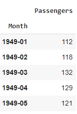
Checking for some values of the data.

data.head()

Output:

Plotting the data.

data.plot(figsize=(14,8), title='alcohol data series')

Output:

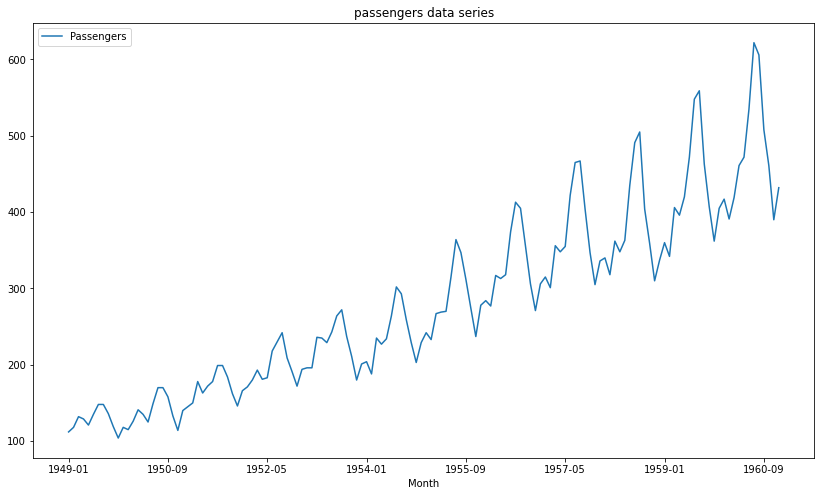
Here we can see that the data we are using is non-stationary because the number of passengers is integrated positively with time.

Now that we have all the things we require, we can perform our test on the time series.

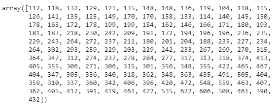
Taking out the passengers number as a series.

series = data['Passengers'].values
series

Output:

Performing the ADF test on the series:

# ADF Test
result = adfuller(series, autolag='AIC')

Extracting the values from the results:

print('ADF Statistic: %f' % result[0])

print('p-value: %f' % result[1])

print('Critical Values:')

for key, value in result[4].items():
    print('\t%s: %.3f' % (key, value))
if result[0] < result[4]["5%"]:
    print ("Reject Ho - Time Series is Stationary")
else:
    print ("Failed to Reject Ho - Time Series is Non-Stationary")

Output:

Here in the results, we can see that the p-value for time series is greater than 0.05, and we can say we fail to reject the null hypothesis and the time series is non-stationary. 

Now, let’s check the test for stationary data.

Loading the data.

path = '/content/drive/MyDrive/Yugesh/LSTM Univarient Single Step Style/temprature.xlsx'
data = pd.read_excel(path, index_col='Date')

Checking for some head values of the data:

data.head()

Output:

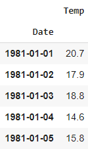
Here we can see that the data has the average temperature values for every day.

Plotting the data.

data.plot(figsize=(14,8), title='temperature data series')

Output:

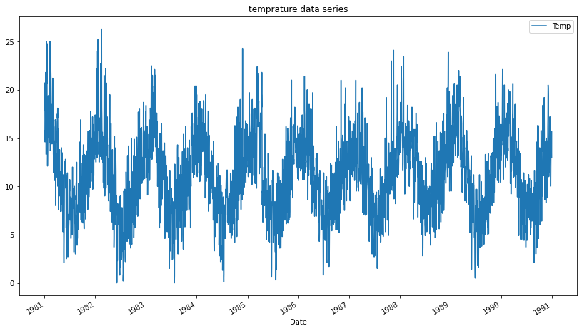
Here we can see that in the data, the larger value follows the next smaller value throughout the time series, so we can say the time series is stationary and check it with the ADF test.

Extracting temperature in a series.

series = data['Temp'].values
series

Output:

Performing ADF test.

result = adfuller(series, autolag='AIC')

Checking the results:

print('ADF Statistic: %f' % result[0])

print('p-value: %f' % result[1])

print('Critical Values:')

for key, value in result[4].items():
    print('\t%s: %.3f' % (key, value))
if result[0] > result[4]["5%"]:
    print ("Reject Ho - Time Series is Stationary")
else:
    print ("Failed to Reject Ho - Time Series is Stationary")

Output:

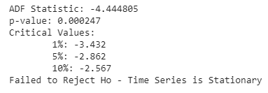
In the results, we can see that the p-value obtained from the test is less than 0.05 so we are going to reject the null hypothesis “Time series is stationary”, that means the time series is non-stationary.

In the article, we have seen why we need to perform the ADF test and the algorithms that the ADF and dickey-fuller test follow to make inferences about any time series. Statsmodel is one of the packages which allows us to perform many kinds of tests and analysis regarding time series analysis.

Popular Posts

• SARIMAX in Python
• Metrics For Time Series Forecasting
• Time Series Feature Engineering
• How To Deseasonalize Data
• Time Series Anomaly Detection Python