In machine learning, the aim is to create algorithms that can learn and predict a required target output from the learnings. To achieve this, the learning algorithm is presented and fed with some examples it can train and learn from to achieve the intended relation of input and output values. Then the learner, a model, in this case, is intended to approximate the correct output, even for examples that have been unseen during the training phase. Without any additional assumptions, problems cannot be solved since unseen situations might have an arbitrary output value. The necessary assumptions about the nature of the target function values are subsumed in the phrase inductive bias. Inductive Bias, also sometimes known as learning bias, is a predictive learning algorithm that uses a set of assumptions that the learner uses to predict outputs of given inputs that it has not encountered yet.
It can also be defined as the process of learning general principles from the data based on specific instances; in other words, it’s what any machine learning algorithm does when it produces a prediction for an unseen test instance based on a definite number of training instances. Inductive bias describes the tendency for a system to prefer a certain set of assumptions over others within the observed data. Without inductive bias introduced, a learner model cannot differentiate or make decisions from observed samples to new samples, and this process is better than random guessing.
Every machine learning algorithm used in practice to date, from the nearest neighbors to gradient boosting machines, come with their own set of inductive biases, such learning algorithms at times possess a bias to learn about similar items or close in terms of attributes to one another in a feature space and hence they are more likely to be classified in the same class. Linear models such as logistic regression assume that a linear boundary can always separate the classes, although this being a hard bias, as the model cannot learn anything else.
Algebraic expressions are usually compact and present us with explicit interpretations and generalize assumptions well. However, finding such algebraic expressions is a difficult task. Symbolic regression comes to the rescue as one of the options. It is a supervised machine learning technique that assembles analytic functions to create a model for a given dataset. However, genetic algorithms are traditionally used, which are essentially brute force procedures that scale exponentially with input variables and operators. On the other hand, deep learning methods allow efficient training of complex models on a high dimensional dataset. However, these learned models are typically black boxes and can be difficult to interpret.
About Symbolic Models Framework with Inductive Biases
Symbolic Model Framework proposes a general framework to leverage the advantages of both traditional deep learning and symbolic regression. As an example, the study of Graph Networks (GNs or GNNs) can be presented, as they have strong and well-motivated inductive biases that are very well suited to complex problems that can be explained. Symbolic regression is applied to fit the different internal parts of the learned model that operate on a reduced size of representations. A Number of symbolic expressions can also be joined together, giving rise to an overall algebraic equation equivalent to the trained Graph Network. The framework can be applied to more such problems as rediscovering force laws, rediscovering Hamiltonians, and a real-world astrophysical challenge, demonstrating that drastic improvements can be made to generalization, and plausible analytical expressions are being made distilled. Not only can it recover the injected closed-form physical laws for the Newtonian and Hamiltonian examples, but it can also derive a new interpretable closed-form analytical expression that can be useful in astrophysics.
The Symbolic Model framework can be summarized as :
- Engineering a deep learning model with a separable internal structure that would provide an inductive bias well matched to the nature of the data. Specifically, Graph Networks can be used as the core inductive bias into the models in the case of interacting particles.
- The model is then trained end-to-end, making use of available data.
- Symbolic expressions are fitted to the distinct functions learned by the created model internally.
- Symbolic expressions then replace functions in the deep model.
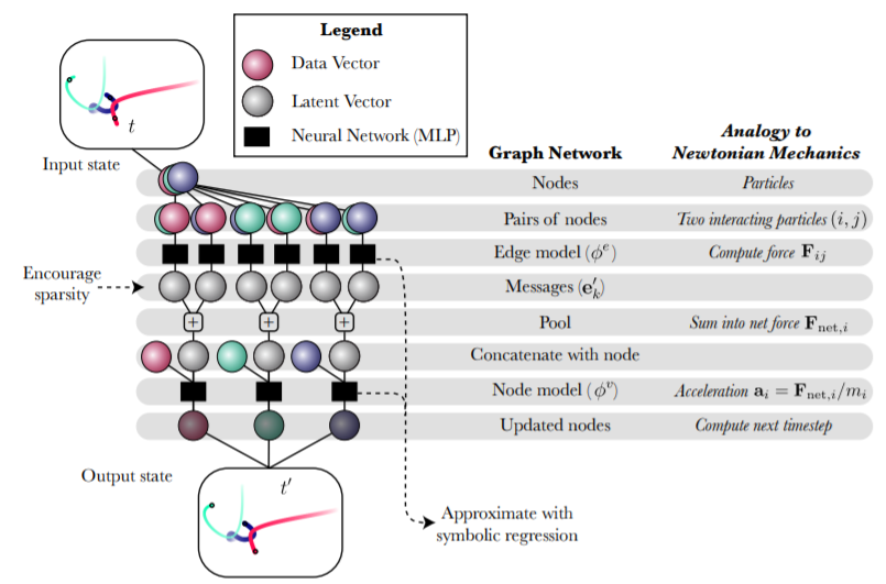
Image source : https://arxiv.org/pdf/2006.11287.pdfGetting Started with Creating a Deep Learning Model With Inductive Bias
This demonstration will try to predict the path dynamics from a simple particle model using Graph Neural Network. We will also try to induce Low Dimensionality for a clearer understanding and predict the dynamic path movement for newly induced particles and extract it to the symbolic equation. The following implementation is inspired by the official demo of the Symbolic model, whose Github repository can be explored here.
Installing the prerequisites
The first step will be to install all the dependencies to create the model, using the following code.
 #Basic pre-reqs:
 import numpy as np
 import os
 import torch
 from torch.autograd import Variable
 from matplotlib import pyplot as plt
 %matplotlib inline
Downloading further prerequisites and then code for simulations and model files, here we will introduce the celluloid library to create interactive animations from our model
!pip install celluloid #to create interactive animations
Installing geometric torch to process our complex model,
 version_nums = torch.__version__.split('.')
 # Torch Geometric seems to always build for *.*.0 of torch :
 version_nums[-1] = '0' + version_nums[-1][1:]
 os.environ['TORCH'] = '.'.join(version_nums)
 !pip install --upgrade torch-scatter -f https://pytorch-geometric.com/whl/torch-${TORCH}.html && pip install --upgrade torch-sparse -f https://pytorch-geometric.com/whl/torch-${TORCH}.html && pip install --upgrade torch-geometric
 #importing the particle model and simulation model
 !wget https://raw.githubusercontent.com/anon928374/gn/master/models.py -O models.py
 !wget https://raw.githubusercontent.com/anon928374/gn/master/simulate.py -O simulate.py
 #calling model and simulation environment
 import models
 import simulate
As this would require heavy processing, make sure you are making use of a GPU
torch.ones(1).cuda() #calling GPU
Now we will create our simulation and set the parameters for it:
 # Number of simulations to run :
 ns = 10000
 # Potential
 sim = 'spring'
 # Number of nodes
 n = 4
 # Dimension
 dim = 2
 # Number of time steps
 nt = 1000
 #Standard simulation sets:
 n_set = [4, 8]
 sim_sets = [
  {'sim': 'r1', 'dt': [5e-3], 'nt': [1000], 'n': n_set, 'dim': [2, 3]},
  {'sim': 'r2', 'dt': [1e-3], 'nt': [1000], 'n': n_set, 'dim': [2, 3]},
  {'sim': 'spring', 'dt': [1e-2], 'nt': [1000], 'n': n_set, 'dim': [2, 3]},
  {'sim': 'string', 'dt': [1e-2], 'nt': [1000], 'n': [30], 'dim': [2]},
  {'sim': 'charge', 'dt': [1e-3], 'nt': [1000], 'n': n_set, 'dim': [2, 3]},
  {'sim': 'superposition', 'dt': [1e-3], 'nt': [1000], 'n': n_set, 'dim': [2, 3]},
  {'sim': 'damped', 'dt': [2e-2], 'nt': [1000], 'n': n_set, 'dim': [2, 3]},
  {'sim': 'discontinuous', 'dt': [1e-2], 'nt': [1000], 'n': n_set, 'dim': [2, 3]},
 ]
 #Select the hand-tuned dt value for a smooth simulation
 # (since scales are different in each potential):
 dt = [ss['dt'][0] for ss in sim_sets if ss['sim'] == sim][0]
 title = '{}_n={}_dim={}_nt={}_dt={}'.format(sim, n, dim, nt, dt)
 print('Running on', title)
Calling our simulation dataset and setting the animation :
 from simulate import SimulationDataset
 s = SimulationDataset(sim, n=n, dim=dim, nt=nt//2, dt=dt)
 base_str = './'
 data_str = title
 s.simulate(ns)
Checking the shape of the called dataset,
 data = s.data
 s.data.shape
Output :
(10000, 500, 4, 6)
Synthesizing the set animation into action,
s.plot(0, animate=True, plot_size=False)
We will get the following interactive animation with control bar from celluloid :

Further tuning our animations and making use of deep neural networks for prediction,
 accel_data = s.get_acceleration() # adding Depth to our animations
 X = torch.from_numpy(np.concatenate([s.data[:, i] for i in range(0, s.data.shape[1], 5)]))
 y = torch.from_numpy(np.concatenate([accel_data[:, i] for i in range(0, s.data.shape[1], 5)]))
 #dividing dataset into train and test
 from sklearn.model_selection import train_test_split
 X_train, X_test, y_train, y_test = train_test_split(X, y, shuffle=False)
 #adding optimizers and creating the graph neural network
 import torch
 from torch import nn
 from torch.functional import F
 from torch.optim import Adam
 from torch_geometric.nn import MetaLayer, MessagePassing
 from models import OGN, varOGN, make_packer, make_unpacker, get_edge_index
 aggr = 'add'
 hidden = 300
 test = '_l1_'
 #This test applies an explicit bottleneck:
 msg_dim = 100
 n_f = data.shape[3]
 #importing Dataloader for feeding input data
 from torch_geometric.data import Data, DataLoader
 from models import get_edge_index
 edge_index = get_edge_index(n, sim)
 if test == '_kl_':
     ogn = varOGN(n_f, msg_dim, dim, dt=0.1, hidden=hidden, edge_index=get_edge_index(n, sim), aggr=aggr).cuda()
 else:
     ogn = OGN(n_f, msg_dim, dim, dt=0.1, hidden=hidden, edge_index=get_edge_index(n, sim), aggr=aggr).cuda()
 messages_over_time = []
 ogn = ogn.cuda()
 #generating the tesors
 _q = Data(
     x=X_train[0].cuda(),
     edge_index=edge_index.cuda(),
     y=y_train[0].cuda())
 ogn(_q.x, _q.edge_index), ogn.just_derivative(_q).shape, _q.y.shape, ogn.loss(_q),
 Output :
 (tensor([[ 0.0231,  0.0075],
          [ 0.0269,  0.0156],
          [ 0.0383, -0.0070],
          [ 0.0295,  0.0047]], device='cuda:0', grad_fn=<AddmmBackward>),
  torch.Size([4, 2]),
  torch.Size([4, 2]),
  tensor(24.7884, device='cuda:0', grad_fn=<SumBackward0>))
 #setting the batch size
 batch = int(64 * (4 / n)**2)
 trainloader = DataLoader(
     [Data(
         Variable(X_train[i]),
         edge_index=edge_index,
         y=Variable(y_train[i])) for i in range(len(y_train))],
     batch_size=batch,
     shuffle=True
 )
 testloader = DataLoader(
     [Data(
         X_test[i],
         edge_index=edge_index,
         y=y_test[i]) for i in range(len(y_test))],
     batch_size=1024,
     shuffle=True
 )
 from torch.optim.lr_scheduler import ReduceLROnPlateau, OneCycleLR
 Defining loss function for the graph neural network.
 #defining loss function
 def new_loss(self, g, augment=True, square=False):
     if square:
         return torch.sum((g.y - self.just_derivative(g, augment=augment))**2)
     else:
         base_loss = torch.sum(torch.abs(g.y - self.just_derivative(g, augment=augment)))
         if test in ['_l1_', '_kl_']:
             s1 = g.x[self.edge_index[0]]
             s2 = g.x[self.edge_index[1]]
             if test == '_l1_':
                 m12 = self.message(s1, s2)
                 regularization = 1e-2
                 #Want one loss value per row of g.y:
                 normalized_l05 = torch.sum(torch.abs(m12))
                 return base_loss, regularization * batch * normalized_l05 / n**2 * n
             elif test == '_kl_':
                 regularization = 1
                 #Want one loss value per row of g.y:
                 tmp = torch.cat([s1, s2], dim=1)  # tmp has shape [E, 2 * in_channels]
                 raw_msg = self.msg_fnc(tmp)
                 mu = raw_msg[:, 0::2]
                 logvar = raw_msg[:, 1::2]
                 full_kl = torch.sum(torch.exp(logvar) + mu**2 - logvar)/2.0
                 return base_loss, regularization * batch * full_kl / n**2 * n
         return base_loss
 Setting optimizers and number of epochs to train our Graph Neural Network.
 init_lr = 1e-3
 opt = torch.optim.Adam(ogn.parameters(), lr=init_lr, weight_decay=1e-8)
 # total_epochs = 200
 total_epochs = 30
 batch_per_epoch = int(1000*10 / (batch/32.0))
 sched = OneCycleLR(opt, max_lr=init_lr,
                    steps_per_epoch=batch_per_epoch,#len(trainloader),
                    epochs=total_epochs, final_div_factor=1e5)
 batch_per_epoch
 from tqdm import tqdm
 import numpy as onp
 onp.random.seed(0)
 test_idxes = onp.random.randint(0, len(X_test), 1000)
 #Record messages over test dataset here:
 newtestloader = DataLoader(
     [Data(
         X_test[i],
         edge_index=edge_index,
         y=y_test[i]) for i in test_idxes],
     batch_size=len(X_test),
     shuffle=False
 )
Setting our model equation for prediction,
 import numpy as onp
 import pandas as pd
 def get_messages(ogn):
     def get_message_info(tmp):
         ogn.cpu()
         s1 = tmp.x[tmp.edge_index[0]]
         s2 = tmp.x[tmp.edge_index[1]]
         tmp = torch.cat([s1, s2], dim=1)  # tmp has shape [E, 2 * in_channels]
         if test == '_kl_':
             raw_msg = ogn.msg_fnc(tmp)
             mu = raw_msg[:, 0::2]
             logvar = raw_msg[:, 1::2]
             m12 = mu
         else:
             m12 = ogn.msg_fnc(tmp)
         all_messages = torch.cat((
             s1,
             s2,
             m12), dim=1)
         if dim == 2:
             columns = [elem%(k) for k in range(1, 3) for elem in 'x%d y%d vx%d vy%d q%d m%d'.split(' ')]
             columns += ['e%d'%(k,) for k in range(msg_dim)]
         elif dim == 3:
             columns = [elem%(k) for k in range(1, 3) for elem in 'x%d y%d z%d vx%d vy%d vz%d q%d m%d'.split(' ')]
             columns += ['e%d'%(k,) for k in range(msg_dim)]
         return pd.DataFrame(
             data=all_messages.cpu().detach().numpy(),
             columns=columns
         )
     msg_info = []
     for i, g in enumerate(newtestloader):
         msg_info.append(get_message_info(g))
     msg_info = pd.concat(msg_info)
     msg_info['dx'] = msg_info.x1 - msg_info.x2
     msg_info['dy'] = msg_info.y1 - msg_info.y2
     if dim == 2:
         msg_info['r'] = np.sqrt(
             (msg_info.dx)**2 + (msg_info.dy)**2
         )
     elif dim == 3:
         msg_info['dz'] = msg_info.z1 - msg_info.z2
         msg_info['r'] = np.sqrt(
             (msg_info.dx)**2 + (msg_info.dy)**2 + (msg_info.dz)**2
         )
     return msg_info
 #importing recorded model
 recorded_models = []
Training our GNN Model:
 for epoch in tqdm(range(epoch, total_epochs)):
     ogn.cuda()
     total_loss = 0.0
     i = 0
     num_items = 0
     while i < batch_per_epoch:
         for ginput in trainloader:
             if i >= batch_per_epoch:
                 break
             opt.zero_grad()
             ginput.x = ginput.x.cuda()
             ginput.y = ginput.y.cuda()
             ginput.edge_index = ginput.edge_index.cuda()
             ginput.batch = ginput.batch.cuda()
             if test in ['_l1_', '_kl_']:
                 loss, reg = new_loss(ogn, ginput, square=False)
                 ((loss + reg)/int(ginput.batch[-1]+1)).backward()
             else:
                 loss = ogn.loss(ginput, square=False)
                 (loss/int(ginput.batch[-1]+1)).backward()
             opt.step()
             sched.step()
             total_loss += loss.item()
             i += 1
             num_items += int(ginput.batch[-1]+1)
     cur_loss = total_loss/num_items
     print(cur_loss)
     cur_msgs = get_messages(ogn)
     cur_msgs['epoch'] = epoch
     cur_msgs['loss'] = cur_loss
     messages_over_time.append(cur_msgs)
     ogn.cpu()
     from copy import deepcopy as copy
     recorded_models.append(ogn.state_dict())
Epoch Output :
  0%|          | 0/30 [00:00<?, ?it/s]12.383322237300872
   7%|▋         | 2/30 [01:50<25:52, 55.44s/it]8.476871449041367
  10%|█         | 3/30 [02:46<24:56, 55.42s/it]6.120438998270035
  13%|█▎        | 4/30 [03:41<24:00, 55.42s/it]5.34595146484375
  17%|█▋        | 5/30 [04:37<23:06, 55.44s/it]4.251027070164681
  20%|██        | 6/30 [05:32<22:11, 55.47s/it]3.295241960835457
  23%|██▎       | 7/30 [06:28<21:16, 55.50s/it]2.725217816901207
  27%|██▋       | 8/30 [07:24<20:22, 55.58s/it]2.4214660188436508
  30%|███       | 9/30 [08:19<19:27, 55.62s/it]2.2335157041072846
  33%|███▎      | 10/30 [09:15<18:33, 55.66s/it]2.0471408730864527
  37%|███▋      | 11/30 [10:11<17:37, 55.64s/it]1.904685971081257
  40%|████      | 12/30 [11:06<16:41, 55.66s/it]1.7552172343373298
  43%|████▎     | 13/30 [12:02<15:46, 55.70s/it]1.5958639140605926
  47%|████▋     | 14/30 [12:58<14:51, 55.73s/it]1.4858177517175675
  50%|█████     | 15/30 [13:54<13:57, 55.82s/it]1.401456927740574
  53%|█████▎    | 16/30 [14:50<13:03, 55.97s/it]1.2299495659947395
  57%|█████▋    | 17/30 [15:46<12:07, 55.97s/it]1.1393675281226634
  60%|██████    | 18/30 [16:42<11:11, 55.93s/it]1.0435665905714036
  63%|██████▎   | 19/30 [17:38<10:15, 55.91s/it]0.9252723445832729
  67%|██████▋   | 20/30 [18:34<09:18, 55.90s/it]0.7918352241277695
  70%|███████   | 21/30 [19:30<08:22, 55.89s/it]0.7148197756946086
  73%|███████▎  | 22/30 [20:25<07:27, 55.88s/it]0.6202942582428456
  77%|███████▋  | 23/30 [21:21<06:30, 55.85s/it]0.5343491077363491
  80%|████████  | 24/30 [22:17<05:35, 55.85s/it]0.453341006103158
  83%|████████▎ | 25/30 [23:13<04:39, 55.84s/it]0.39567755371034147
  87%|████████▋ | 26/30 [24:09<03:43, 55.83s/it]0.3454551042586565
  90%|█████████ | 27/30 [25:04<02:47, 55.71s/it]0.30814071524441244
  93%|█████████▎| 28/30 [26:00<01:51, 55.68s/it]0.2823368747919798
  97%|█████████▋| 29/30 [26:55<00:55, 55.57s/it]0.26827718360722064
 100%|██████████| 30/30 [27:51<00:00, 55.70s/it]0.2626891137778759
Predicting new Particles & Plotting our simulation from the trained model,
 #setting color for predicted particles
 from simulate import make_transparent_color
 from scipy.integrate import odeint
 Introducing Different Point of view to observe predictions :
 fig, ax = plt.subplots(1, 2, figsize=(8, 4))
 camera = Camera(fig)
 for current_model in [-1] + [1, 34, 67, 100, 133, 166, 199]:
     i = 4 #Use this simulation
     if current_model > len(recorded_models):
         continue
     #Truth:
     cutoff_time = 300
     times = onp.array(s.times)[:cutoff_time]
     x_times = onp.array(data[i, :cutoff_time])
     masses = x_times[:, :, -1]
     length_of_tail = 75
     #Learned:
     e = edge_index.cuda()
     ogn.cpu()
     if current_model > -1:
         ogn.load_state_dict(recorded_models[current_model])
     else:
         # Random model!
         ogn = OGN(n_f, msg_dim, dim, dt=0.1, hidden=hidden, edge_index=get_edge_index(n, sim), aggr=aggr).cuda()
     ogn.cuda()
     def odefunc(y, t=None):
         y = y.reshape(4, 6).astype(np.float32)
         cur = Data(
             x=torch.from_numpy(y).cuda(),
             edge_index=e
         )
         dx = y[:, 2:4]
         dv = ogn.just_derivative(cur).cpu().detach().numpy()
         dother = np.zeros_like(dx)
         return np.concatenate((dx, dv, dother), axis=1).ravel()
     datai = odeint(odefunc, (onp.asarray(x_times[0]).ravel()), times).reshape(-1, 4, 6)
     x_times2 = onp.array(datai)
     d_idx = 10
     for t_idx in range(d_idx, cutoff_time, d_idx):
         start = max([0, t_idx-length_of_tail])
         ctimes = times[start:t_idx]
         cx_times = x_times[start:t_idx]
         cx_times2 = x_times2[start:t_idx]
         for j in range(n):
             rgba = make_transparent_color(len(ctimes), j/n)
             ax[0].scatter(cx_times[:, j, 0], cx_times[:, j, 1], color=rgba)
             ax[1].scatter(cx_times2[:, j, 0], cx_times2[:, j, 1], color=rgba)
             black_rgba = rgba
             black_rgba[:, :3] = 0.75
             ax[1].scatter(cx_times[:, j, 0], cx_times[:, j, 1], color=black_rgba, zorder=-1)
         for k in range(2):
             ax[k].set_xlim(-1, 3)
             ax[k].set_ylim(-3, 1)
         plt.tight_layout()
         camera.snap()
 # camera.animate().save('multiple_animations_with_comparison.mp4')
 from IPython.display import HTML
 HTML(camera.animate().to_jshtml())
Final Output :
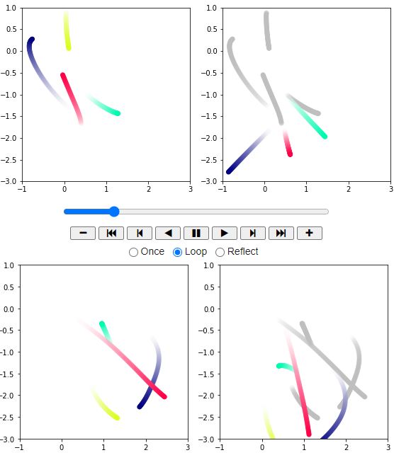
As we can observe, the predicted particles and their path are indicated with a transparent grey color!
EndNotes
This article tried to explore and learn about Symbolic Models with Inductive Biases and how they can be created using Deep Learning Networks. You can find the implemented code in the following colab notebook here.


