Published on August 24, 2021
In AI Trends

Why Decompose a Time Series, and How?

Components of time series are level, trend, season and residual/noise. breaking a time series into its component is decompose a time series.

By Yugesh Verma

In time series analysis for forecasting new values, it is very important to know about the past data. More formally, we can say it is very important to know about the patterns which are followed by the values with time. There can be many reasons which cause our forecasted values to fall in the wrong direction. Basically, a time series consists of four components. Variation of those components causes the change in the pattern of the time series. These components are:

Level: It is the main value that goes on average with time.
Trend: The trend is the value that causes increasing or decreasing patterns in a time series.
Seasonality: This is a cyclic event that occurs in time series for a short time and causes the increasing or decreasing patterns for a short time in a time series.
Noise: These are the random variations in the time series.

The combination of those components with time causes the formation of a time series. Most time series consists of the level and noise/residual and the trend or seasonality are the optional values. They may take part or they may not.

If seasonality and trend are part of the time series then there will be effects in the forecast value. As the pattern of the forecasted time series can be different from the older time series.

The combination of the components in time series can be of two types:

Additive
Multiplicative

Additive time series

if the components of the time series are added together to make the time series. Then the time series is called the additive time series. By visualization, we can say the time series is additive if the increasing or decreasing pattern of the time series is similar throughout the series. The mathematical function of any additive time series can be represented by:

y(t) = level + Trend + seasonality + noise

Multiplicative time series

If the components of the time series are multiplicative together, then the time series is called the multiplicative time series. By visualization, if the time series is having exponential growth or decrement with time then the time series can be considered as the multiplicative time series. The mathematical function of the Multiplicative time series can be represented as.

y(t) = Level * Trend * seasonality * Noise

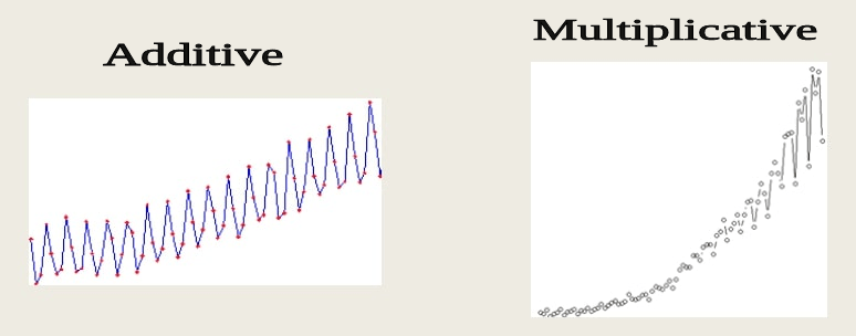
The image below represents the additive and multiplicative time series.

Image source

In the above image, we can see the difference in the growth of values. In additive, it is quite slower and has a proper trend but on the other hand, we can see that the time series is growing exponentially with the time

Instead of knowing the type of time series, it is better to know about the component of the time series. As we earlier discussed, the time series is the composition of level, trend, season and residuals. It is much better to know all the components in a time series for better understanding and making a model more accurate for better forecasting values.

In this article, we will see how we can measure these components in any time series by decomposing a time series in its components.

Here in the process, I am using the airline-passenger dataset which consists of the count of passengers in the airline with the date values.

Importing the libraries:

import pandas as pd
import numpy as np

Reading the dataset

path = '/content/drive/MyDrive/Yugesh/deseasonalizing time series/AirPassengers.csv'
data = pd.read_csv(path, index_col='Month')

Checking for the 20 heads of the dataset.

data.head(20)

Output:

Index of the dataset

data.index

Output:

Here we can see the name of the index is Month and the length of the data is 144, in 20 heads we have seen that the column name of the time series is Passengers.

Plotting the data:

import matplotlib.pyplot as plt
plt.rcParams["figure.figsize"] = (15,10)
data.plot()
plt.show()

Output:

Here we can clearly see that there is a trend in the time series and there may be a chance to present seasonality in the time series.

To check for all of the components in the time series by decomposition, we can use the python library statsmodel provided seasonal_decompose package.

from statsmodels.tsa.seasonal import seasonal_decompose
data = data.asfreq('MS')
decompose_data = seasonal_decompose(data, model="multiplicative")
decompose_data.plot()
plt.show()

Output:

Here we can clearly see by visualization that there is trend and season is present in the time series also the residual is showing high variability.

We can check it more with additives.

decompose_data = seasonal_decompose(data, model="additive")
decompose_data.plot()
plt.show()

Output:

Here we can clearly see the variability of the residual in the additive model.

We can also visualize the components separately.

Visualizing the observed values.

level = decompose_data.observed
level.plot()

Output:

Visualizing the trend.

trend=decompose_data.trend
trend.plot()

Output:

Visualizing the seasonality.

seasonality = decompose_data.seasonal
seasonality.plot()

Output:

Visualizing the residual.

residual = decompose_data.resid
residual.plot()

Output:

We also save the components in tabular form by simply concatenating them

component = pd.concat([level, trend, seasonality, residual],axis=1)
component.tail(10)

Output:

Here in the article, we have gone through the procedure of decomposition of a time series. In time series if the components are available in uneven amounts then it can cause the model to predict wrong values. To improve the quality of the prediction we can perform detrending, deseasonalizing and perform some smoothing methods on it. I have covered some methods of cleaning a time series from its components in these articles:

Also, some more information is provided regarding tests we need to perform in time series modelling.

After analyzing and performing all the required analyses in the time series we can go through the modelling of time series for which these articles can help a reader.

I encourage you to go through the article and use it in real-world time series data. These all are the basic articles to perform time series analysis and are very easy to perform going through all you can master in time series analysis.

References:

Seasonal decomposition using moving averages.
Google Colab Notebook for above codes

📣 Want to advertise in AIM? Book here

Yugesh Verma

Yugesh is a graduate in automobile engineering and worked as a data analyst intern. He completed several Data Science projects. He has a strong interest in Deep Learning and writing blogs on data science and machine learning.