The purpose of classification or discriminant analysis is to analyze the observation-based set of measurements to classify the objects into one of several groups or classes. Based on the loss function the discriminant analysis is categorized as Linear Discriminant Analysis and Quadratic Discriminant Analysis. These discriminant analysis have some flaws which can be mitigated by regularization. So in this article, we are going to discuss how discriminant analysis can be regularized. Following are the topics to be covered.
Table of contents
- Brief description of LDA and QDA
- Regularized Discriminant Analysis
- Implementation in python
Let’s first briefly discuss Linear and Quadratic Discriminant Analysis.
Brief description of LDA and QDA
Linear Discriminant Analysis or Discriminant Function Analysis is a dimensionality reduction technique that is commonly used for supervised classification problems. It uses a linear line for explaining the relationship between the dependent variable and the explanatory variable. It is used for modelling differences in groups i.e. separating two or more classes. It is used to project the features in a higher dimension space into a lower dimension space. In LDA there are a few assumptions that are considered by the learner.
- The data has a gaussian distribution
- There are no outliers in the data
- There is the same variance in the entire data
Quadratic discriminant analysis is quite similar to Linear discriminant analysis as both work on the Bayes theorem of probability except QDA does not assume that the data have equal mean and covariance for all the classes. Therefore need to calculate the mean and covariance separately. It uses a quadratic curve to explain the relationship between the dependent variable and the independent variable. There are a few assumptions that are to be considered before implementing the QDA.
- The explanatory classes should have different covariance.
- The response classes are normally distributed with a class-specific mean and class-specific covariance.
Both of the discriminant analysis techniques are biased while generating the eigenvalues and eigenvectors associated with them. This biasing phenomenon on discriminant analysis has the net effect of exaggerating the importance of the low-variance subspace spanned by the eigenvectors corresponding to the smallest sample eigenvalues. Thus, the majority of the variance in estimating the discriminant scores (which are used in data classification) is associated with directions of low sample variance in the measurement space.
Are you looking for a complete repository of Python libraries used in data science, check out here.
Regularized Discriminant Analysis
Since regularization techniques have been highly successful in the solution of ill-posed and poorly-posed inverse problems so to mitigate this problem the most reliable way is to use the regularization technique.
- A poorly posed problem occurs when the number of parameters to be estimated is comparable to the number of observations.
- Similarly,ill-posed if that number exceeds the sample size.
In these cases the parameter estimates can be highly unstable, giving rise to high variance. Regularization would help to improve the estimates by shifting them away from their sample-based values towards values that are more physically valid; this would be achieved by applying shrinkage to each class.
While regularization reduces the variance associated with the sample-based estimate, it may also increase bias. This process known as bias-variance trade-off is generally controlled by one or more degree-of-belief parameters that determine how strongly biasing towards “plausible” values of population parameters takes place.
Whenever the sample size is not significantly greater than the dimension of measurement space for any class, Quantitative discriminant analysis (QDA) is ill-posed. Typically, regularization is applied to a discriminant analysis by replacing the individual class sample covariance matrices with the average weights assigned to the eigenvalues.
This applies a considerable degree of regularization by substantially reducing the number of parameters to be estimated. The regularization parameter () which is added to the equation of QDA and LDA takes a value between 0 to 1. It controls the degree of shrinkage of the individual class covariance matrix estimates toward the pooled estimate. Values between these limits represent degrees of regularization.
Let’s have a look at the implementation of this concept in python on a dataset.
Implementation in python
Let’s mitigate the flaws of the Linear Discriminant Analysis (LDA) in python and build a Regularized Discriminant Analysis (RDA) learner.
Import necessary libraries
import numpy as np
import pandas as pd
import matplotlib.pyplot as plt
import seaborn as sns
from sklearn.model_selection import train_test_split,cross_val_score,RepeatedStratifiedKFold,GridSearchCV
from sklearn.discriminant_analysis import LinearDiscriminantAnalysis
from sklearn.metrics import ConfusionMatrixDisplay,precision_score,recall_score,confusion_matrix
from imblearn.over_sampling import SMOTE
Read and pre-processing the data
df=pd.read_csv("/content/drive/MyDrive/Datasets/healthcare-dataset-stroke-data.csv")
print("Records=",df.shape[0],"\nFeatures=",df.shape[1])
df.head()

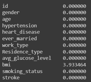
The contains a total of 12 features including the dependent variable in which few are categorical and needed to be encoded before the fitting process. The data is related to healthcare, it contains records for the patients who have suffered from a heart attack. While the analysis found some missing values in the “BMI” feature which is mitigated by dropping the missing values since they can’t be synthesized.
Mitigating missing values
df.isnull().sum()/len(df)*100
df.dropna(axis=0,inplace=True)
Creating dummies
df_pre=pd.get_dummies(df,drop_first=True)
Need to drop the first to save the learner from the dummy variable trap.
Split the data into training and test for the learning and testing phase of the learner. Use the standard 70:30 ratio for the split.
X=df_pre.drop(['stroke'],axis=1)
y=df_pre['stroke']
X_train, X_test, y_train, y_test = train_test_split(X, y, test_size=0.30, random_state=42)
Build the LDA
LDA = LinearDiscriminantAnalysis()
LDA.fit_transform(X_train,y_train)
X_test['predictions']=LDA.predict(X_test)
ConfusionMatrixDisplay.from_predictions(y_test, X_test['predictions'])
plt.show()

tn, fp, fn, tp = confusion_matrix(list(y_test), list(X_test['predictions']), labels=[0, 1]).ravel()

print('True Positive :', tp)
print('True Negative :', tn)
print('False Positive :', fp)
print('False Negative :', fn)
print("Precision score",precision_score(y_test,X_test['predictions']))

The learner has 35% precision in predicting the patient would be having a heart attack in future which is pretty bad. Let’s analyze what’s wrong with the learner.
Regularizing and shrinking the LDA
Starting with the analysis of the target variable.
df_pre['stroke'].value_counts()
0    4700
1     209
As observed by the value count of the dependent variable the data is imbalanced as the quantity of 1’s is approx 4% of the total dependent variable. So, it needs to be balanced for the learner to be a good predictor.
Balancing the dependent variable
There are two ways by which the data can be synthesized: one by oversampling and the second, by undersampling. In this scenario, oversampling is better which will synthesize the lesser category linear interpolation.
oversample = SMOTE()
X_smote, y_smote = oversample.fit_resample(X, y)
Xs_train, Xs_test, ys_train, ys_test = train_test_split(X_smote, y_smote, test_size=0.30, random_state=42)
The imbalance is mitigated by using the Synthetic Minority Oversampling Technique (SMOTE) but this will not help much we also need to regularize the leaner by using the GridSearchCV which will find the best parameters for the learner and add a penalty to the solver which will shrink the eigenvalue i.e regularization.
cv = RepeatedStratifiedKFold(n_splits=10, n_repeats=3, random_state=42)
grid = dict()
grid['solver'] = ['eigen','lsqr']
grid['shrinkage'] = ['auto',0.2,1,0.3,0.5]
search = GridSearchCV(LDA, grid, scoring='precision', cv=cv, n_jobs=-1)
results = search.fit(Xs_train, ys_train)
print('Precision: %.3f' % results.best_score_)
print('Configuration:',results.best_params_)
Precision: 0.873
Configuration: {'shrinkage': 'auto', 'solver': 'eigen'}
The precision score jumped right from 35% to 87% with the help of regularization and shrinkage of the learner and the best solver for the Linear Discriminant Analysis is ‘eigen’ and the shrinkage method is ‘auto’ which uses the Ledoit-Wolf lemma for finding the shrinkage penalty.
Build the RDA
LDA_final=LinearDiscriminantAnalysis(shrinkage='auto', solver='eigen')
LDA_final.fit_transform(Xs_train,ys_train)
Xs_test['predictions']=LDA_final.predict(Xs_test)
ConfusionMatrixDisplay.from_predictions(ys_test, Xs_test['predictions'])
plt.show()

tn, fp, fn, tp = confusion_matrix(list(ys_test), list(Xs_test['predictions']), labels=[0, 1]).ravel()

print('True Positive :', tp)
print('True Negative :', tn)
print('False Positive :', fp)
print('False Negative :', fn)
print("Precision score",np.round(precision_score(ys_test,Xs_test['predictions']),3))
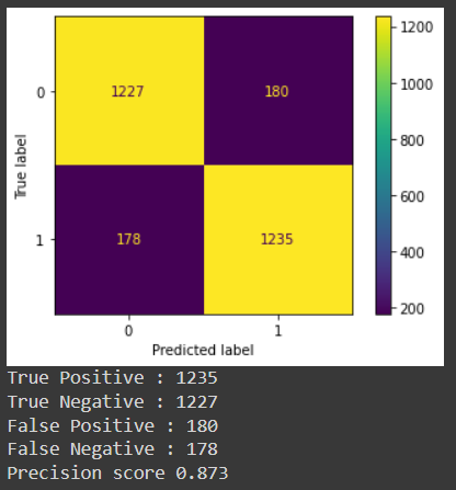
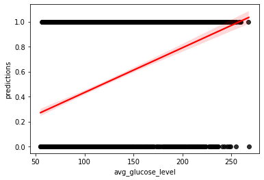
A regression plot for the final learner with a linear relationship line explaining the classification. This learner can be further improved by decreasing the False negatives as they are type2 errors, leaving that to you.
Final Verdict
The method of regularization applied here has the potential to (sometimes dramatically) increase the power of discriminant analysis. With a hands-on implementation of this concept in this article, we could understand Regularized Discriminant Analysis (RDA).


