

Identification of customers based on their choices and other behaviors is an important strategy in any organization. This identification may help in approaching customers with specific offers and products. An organization with a large number of customers may experience difficulty in identifying and placing into a record each customer individually. A huge amount of data processing and automated techniques are involved in extracting insights from the large information collected on customers.
Clustering, an unsupervised technique in machine learning (ML), helps identify customers based on their key characteristics. In this article, we will discuss the identification and segmentation of customers using two clustering techniques – K-Means clustering and hierarchical clustering. We will see the result of clustering when we implement these techniques in Python. Finally, we will discuss the comparison between these two clustering techniques – K-Means and Hierarchical clustering.
The Problem Statement
Imagine a mall which has recorded the details of 200 of its customers through a membership campaign. Now, it has information about customers, including their gender, age, annual income and a spending score. This spending score is given to customers based on their past spending habits from purchases they made from the mall.
Now, suppose the mall is launching a luxurious product and wants to reach out to potential customers who can buy it. Approaching every customer will take a lot of time and will be an expensive exercise. Hence, using the information on customers, the mall may want to segregate customers who have the potential to buy a luxurious product. This problem can be addressed through clustering, where we can place customers into different segments and identify potential customers.
We can represent the customer on a two-dimensional Euclidean space where X-axis will represent the annual income of customers, and Y-axis will represent the spending score of customers. After representing each of the customers on this plane, using a clustering technique, we can form the groups of customers. Now, on the basis of their income and spending score, we can identify the group of customers who have the potential to buy a luxurious product.
Clustering Of Customers
First, we will implement the task using K-Means clustering, then use Hierarchical clustering, and finally, we will explore the comparison between these two techniques, K-Means and Hierarchical clustering. It is expected that you have a basic idea about these two clustering techniques. For more details, you can refer to these two posts:
- Most Popular Clustering Algorithms Used in Machine Learning
- Clustering Techniques Every Data Science Beginner Should Swear By
Customer Segmentation Using K-Means & Hierarchical Clustering
Now, we are going to implement the K-Means clustering technique in segmenting the customers as discussed in the above section. Follow the steps below:
1. Import the basic libraries to read the CSV file and visualize the data
import matplotlib.pyplot as plt
import pandas as pd
2. Read the dataset that is in a CSV file. Define the dataset for the model
dataset = pd.read_csv('Mall_Customers.csv')
X = dataset.iloc[:, [3, 4]].values
3. In order to implement the K-Means clustering, we need to find the optimal number of clusters in which customers will be placed. To find the optimal number of clusters for K-Means, the Elbow method is used based on Within-Cluster-Sum-of-Squares (WCSS). For more details, refer to this post.
from sklearn.cluster import KMeans
wcss = []
for i in range(1, 11):
    kmeans = KMeans(n_clusters = i, init = 'k-means++', random_state = 42)
    kmeans.fit(X)
    wcss.append(kmeans.inertia_)
plt.plot(range(1, 11), wcss)
plt.title('Elbow Method')
plt.xlabel('Number of clusters')
plt.ylabel('WCSS')
plt.show()
It will be plotted as given below:
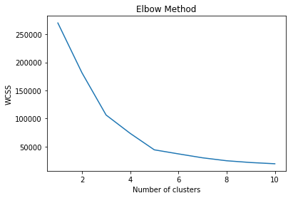
As we can see in the above figure, the above plot is visualized as a hand and we need to identify the location of the elbow on the X-axis. In the above plot, the elbow seems to be on point 5 of X-axis. So, the optimal number of clusters will be 5 for the K-Means algorithm.
4. After finding the optimal number of clusters, fit the K-Means clustering model to the dataset defined in the second step and then predict clusters for each of the data elements. It means it will predict which of the 5 clusters the data item will belong to.
kmeans = KMeans(n_clusters = 5, init = 'k-means++', random_state = 42)
y_kmeans = kmeans.fit_predict(X)
5. When the algorithm predicts a cluster for each of the data items, we need to visualize the result through the plot. For better representation, we need to give each of the clusters a unique colour and name.
plt.figure(figsize=(8,8))
plt.scatter(X[y_kmeans == 0, 0], X[y_kmeans == 0, 1], s = 100, c = 'red', label = 'Standard Customers')
plt.scatter(X[y_kmeans == 1, 0], X[y_kmeans == 1, 1], s = 100, c = 'blue', label = 'Careful Customers')
plt.scatter(X[y_kmeans == 2, 0], X[y_kmeans == 2, 1], s = 100, c = 'green', label = 'Sensible Customers')
plt.scatter(X[y_kmeans == 3, 0], X[y_kmeans == 3, 1], s = 100, c = 'cyan', label = 'Careless Customers')
plt.scatter(X[y_kmeans == 4, 0], X[y_kmeans == 4, 1], s = 100, c = 'magenta', label = 'Target Customers')
plt.title('Clusters of Customers using K-Means Clustering')
plt.xlabel('Annual Income (K$)')
plt.ylabel('Spend Score (1-100)')
plt.legend()
plt.show()
The above plot is given below:
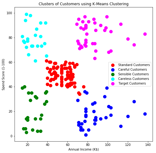
The name of clusters is given based on their income and spending. For example, when referring to a customer with low income and high spending, we have used cyan colour. This group indicates ‘Careless Customer’ since despite having a low income, they spend more. To sell a luxurious product, a person with high income and high spending habits should be targeted. This group of customers is represented in magenta colour in the above diagram.
6. Now the same task will be implemented using Hierarchical clustering. The reading of CSV files and creating a dataset for algorithms will be common as given in the first and second step. In K-Means, the number of optimal clusters was found using the elbow method. In hierarchical clustering, the dendrograms are used for this purpose. The below lines of code plot a dendrogram for our dataset.
import scipy.cluster.hierarchy as sch
plt.figure(figsize=(10,10))
dendrogram = sch.dendrogram(sch.linkage(X, method = 'ward'))
plt.title('Dendrogram')
plt.xlabel('Customers')
plt.ylabel('Euclidean distances')
plt.show()
This dendrogram plot is visualized as:
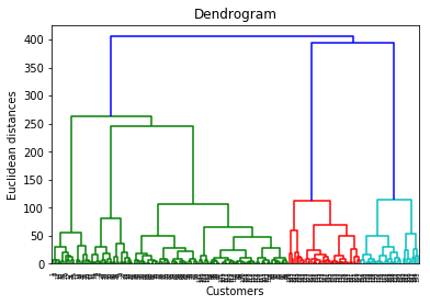
If you are aware of this method, you can see in the above diagrams. The combination of 5 lines are not joined on the Y-axis from 100 to 240, for about 140 units. So, the optimal number of clusters will be 5 for hierarchical clustering.
7. Now we train the hierarchical clustering algorithm and predict the cluster for each data point.
from sklearn.cluster import AgglomerativeClustering
hc = AgglomerativeClustering(n_clusters = 5, affinity = 'euclidean', linkage = 'ward')
y_hc = hc.fit_predict(X)
8. Once the algorithm predicts the cluster for each of the data points, it can be visualized now.
# Visualising the clusters

plt.figure(figsize=(8,8))
plt.scatter(X[y_hc == 0, 0], X[y_hc == 0, 1], s = 100, c = 'red', label = 'Careful Customers')
plt.scatter(X[y_hc == 1, 0], X[y_hc == 1, 1], s = 100, c = 'blue', label = 'Standard Customers')
plt.scatter(X[y_hc == 2, 0], X[y_hc == 2, 1], s = 100, c = 'green', label = 'Target Customers')
plt.scatter(X[y_hc == 3, 0], X[y_hc == 3, 1], s = 100, c = 'cyan', label = 'Careless Customers')
plt.scatter(X[y_hc == 4, 0], X[y_hc == 4, 1], s = 100, c = 'magenta', label = 'Sensible Customers')
plt.title('Clusters of customers using Hierarchical Clustering')
plt.xlabel('Annual Income (K$)')
plt.ylabel('Spending Score (1-100)')
plt.legend()
plt.show()
The above plot can be visualized as:
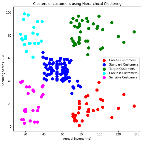
We can see in the above diagram that clustering of customers is almost similar to what was done by K-Means clustering. Only the colour combinations have been changed for differentiating both the diagrams.
Comparison Between K-Means & Hierarchical Clustering
As we have seen in the above section, the results of both the clustering are almost similar to the same dataset. It may be possible that when we have a very large dataset, the shape of clusters may differ a little. However, along with many similarities, these two techniques have some differences also. The below table shows the comparison between K-Means and Hierarchical clustering algorithms based on our implementations.
| K-Means Clustering | Hierarchical Clustering | |
| Category | Centroid based, partition-based | Hierarchical, Agglomerative |
| Method to find the optimal number of clusters | The Elbow method using WCSS | Dendrogram |
| Directional approach | Not any, the only centroid is considered to form clusters | Top-down, bottom-up |
| Python Library | sklearn – KMeans | sklearn-AgglomerativeClustering |