By fitting data to a logistic curve, logistic regression evaluates the connection between many independent factors and a categorical dependent variable and determines the likelihood of an event occurring. The loss function of logistic regression is a logistic loss which classifies based on the maximum likelihood estimation. This likelihood estimation tends to be biassed toward the higher value due to which regularization is required.  This article will focus on understanding the role of L2 regularization in logistic regression. Following are the topics to be covered.

Table of contents

1. Brief about the loss function of logistic regression
2. About L2 regularization
3. Role of L2 regularization in Logistic Regression
4. Implementing L2 regularization

The penalty for failing to fulfil the planned production is referred to as a ‘loss.’ Let’s start with understanding the loss function of logistic regression.

Brief about the loss function of logistic regression

A loss function is a mathematical function that translates a theoretical declaration into a practical proposition. Developing a highly accurate predictor involves continual issue iteration via questioning, modelling the problem using the chosen approach, and testing.

A logistic regression classifier predicts probabilities based on the weights in the training dataset, and the model will update its weights to minimise the difference between its predicted probabilities and the distribution of probabilities in the training data. This calculation is used for a binary prediction known as binary cross-entropy or log loss.

Although this is erroneous, the term “cross-entropy” is occasionally used to refer to the negative log-likelihood of a Bernoulli or softmax distribution. When characterised by a negative log-likelihood, a loss may be defined as a cross-entropy between an empirical distribution produced from the training set and a probability distribution derived from the model. For example, mean squared error is the cross-entropy between an empirical distribution and a Gaussian model.

Are you looking for a complete repository of Python libraries used in data science, check out here.

About L2 regularization

When training a machine learning model, it is easy for the model to become overfitted or under fitted. To circumvent this, regularisation is utilized in machine learning to fit a model to our test set effectively. Regularization techniques aid in reducing the likelihood of overfitting and obtaining an ideal model.

Ridge regularization or L2 normalization is a penalty method which makes all the weight coefficients to be small but not zero. It is done by taking squares of the weights. This means that the mathematical function corresponding to our machine learning model is minimised, and coefficients are computed. Coefficient magnitudes are squared and summed. Ridge Regression accomplishes regularisation by reducing the number of coefficients. Here is the cost function.

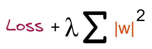
Where,

Loss = sum of squared residuals

λ = penalty for the error

W = slope of the curve

Lambda represents the penalty term in the cost function. We regulate the punishment term by adjusting the values of the penalty function. The greater the penalty, the smaller the size of the coefficients. It reduces the parameters. As a result, it is utilised to prevent multicollinearity and to minimise model complexity through coefficient shrinking.

Need for regularization in Logistic Regression

Regularization is critical in logistic regression modelling. Without regularisation, logistic regression’s asymptotic nature would continue to drive loss towards 0 in large dimensions. As a result, to reduce model complexity, most logistic regression models include either L2 regularisation or early stopping (reducing the number of training steps or the learning rate).

Consider assigning a unique id to each example and mapping each id to its own feature. If no regularisation function is specified, the model will become entirely overfit. Because the model would try and fail to drive loss to zero on all samples, pushing the weights for each indicator feature to +∞ or -∞. This can occur with high-dimensional data with feature crosses when there is a large number of unusual crosses that occur only on a single occurrence.

Role of L2 regularization in Logistic Regression

There is a high chance that the logistic regression overfits when dealing with polynomial data. When there is more than one independent variable it is known as a polynomial. Here is an example of this statement.

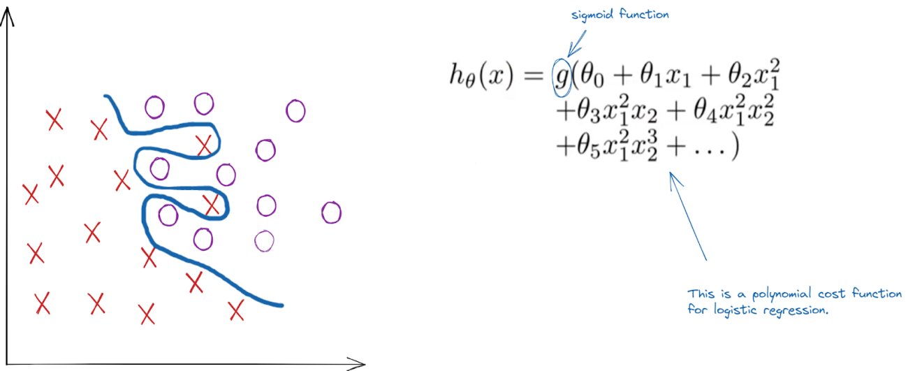
As in the above example, the decision boundary is too complex which indicates that the model is biassed towards the ‘x’ data points. On the right side of the image, a polynomial sigmoid function is mentioned for the logistic regression. So, to regularise the algorithm and make the decision boundary-less complicated need to use a penalty which will restrict the model from being biased. The penalty to be used for the logistic regression is Ridge regularization. The mathematical equation for when using the ridge penalty would be this:

This formula would be integrated with the gradient descent for more advanced optimization of the Regularized Logistic regression.

Implementing L2 regularization

This article uses sklearn logistic regression and the dataset used is related to medical science. The task is to predict the CDH based on the patient’s historical data using an L2 penalty on the Logistic Regression.

Let’s import the necessary libraries

import numpy as np
import pandas as pd
import matplotlib.pyplot as plt

Reading the data and preparing for training by splitting the data into standard ratios of 30:70 for testing and training respectively.

data=pd.read_csv('/content/drive/MyDrive/Datasets/heart.csv')
X=data.drop(['output'],axis=1)
y=data['output']
X_train, X_test, y_train, y_test = train_test_split(X, y, test_size=0.30, random_state=42)

Build the regularized logistic regression

regularized_lr=LogisticRegression(penalty='l2',solver='newton-cg',max_iter=200)
regularized_lr.fit(X_train,y_train)
reg_pred=regularized_lr.predict(X_test)

For using the L2 regularization in the sklearn logistic regression model define the penalty hyperparameter. For this data need to use the ‘newton-cg’ solver because the data is less and any other method would not converge and a maximum iteration of 200 is enough.

print('Precision score',np.round(precision_score(y_test,reg_pred),2))
print('Recall score',np.round(recall_score(y_test,reg_pred),2))
cm_reg = confusion_matrix(y_test, reg_pred, labels=regularized_lr.classes_)
disp_reg = ConfusionMatrixDisplay(confusion_matrix=cm_reg,display_labels=regularized_lr.classes_)
disp_reg.plot()
plt.show()

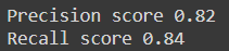
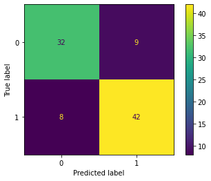
We are getting a precision score of 0.82 which is good in other situations but not in the medical case and similar for recall, a score of 0.84 is good but not in this case. The train data hasn’t been wrangled, and need to standardise the data because all the measurements of the parameters have different units, could also do some feature selection, engineering, etc. So to improve on the model level the primary focus is on the FALSE NEGATIVE  reduction which is currently at 8 because there is a high chance that due to this a patient could die. Well, leave that to you folks.

Conclusions

Regularization is critical in logistic regression modelling. Without regularisation, logistic regression’s asymptotic nature would continue to drive loss towards 0 in large dimensions. With this article, we have understood the implementation and concept of L2 regularization in Logistic Regression.

References

• Link to the above code
• Documentation by sklearn for LR